
As part of the Google Advanced Data Analytics professional certificate program, I acted as a data professional that analyzed HR data to provide recommendations to improve the employee retention rate for Salifort Motors, a fictional company.
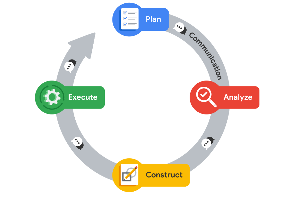
I utilized the PACE workflow to provide structure to data analysis tasks. For each of the stages in the workflow there are questions to be considered to guide the analysis. The PACE workflow is summarized as below:

The questions that a data professional should consider answering are:
1. What are the goals of the project?
· The goals in this project are to analyze the data collected by the HR department and to build a model that predicts whether or not an employee will leave the company.
· If the model can predict employees likely to quit, it might be possible to identify factors that contribute to their leaving.
2. How will the business or operation be affected by the plan?
· It is time-consuming and expensive to find, interview, and hire new employees, increasing employee retention will be beneficial to the company.
· The aim of the project is to analyze the data collected by the HR department and to build a model that predicts whether or not an employee will leave the company in order to strategize how to incentivize the employee to stay in the company.
3. Who are the main stakeholders of the project?
· The main stakeholders are the HR department managers that would like to improve initiatives for employee retention. They collected data from employees in order to gain insights about employee satisfaction.
· The stakeholders would like data-driven suggestions based on understanding of the data to answer their main question: what’s likely to make the employee leave the company?
4. What strategies will be needed?
· As the data professional, I would require to inspect the data to check the data integrity, through exploratory data analysis.
5. How can the data be cleaned and converted into a usable format?
· The data provided is the HR dataset which is a csv file: HR_capstone_dataset.csv.
· The data would need to be checked for missing data and duplicates.
· Examine the class balance of your target variable so as not to overfit/ underfit the models.
· The categorical variables need to be encoded to numerical values in order to fit the models.
· The dataset contains 10 columns providing information about various employee’s satisfaction level. The columns in the dataset are:

Step 1: Gather basic information about the data
Using the info() method, I analyzed the data columns to get information on the number of records, if the columns contained null records and data types of the data.

Step 2: Gather descriptive statistics about the data
Using the describe method, I derived descriptive statistics on numerical columns.

Step 3: Rename columns
There were columns that had typos in their column names i.e. (average_montly hours) and columns which were not in snake case. i.e. (Work_accident). I renamed the column to average_monthly hours and changed the case to work_accident.

Step 4: Check missing values
I used the isna() method to check the number of columns with null values. There were no rows with missing values.

Step 5: Check for duplicates then remove them
I used the duplicated() method to check whether the data had duplicates. There were 3008 rows with duplicate records. I used the drop_duplicates() method to remove the duplicates.


Step 6: Check outliers
I checked the columns for outlier by plotting box plots.

There were outliers in the time_spend_company. I checked the number of rows with outliers by checking the number of rows with tenure of greater than 5 years. The number of rows was 5628.

This shows that the data flagged as outliers were not outliers, these were records which were considerably higher than the average mean of 3.8 years tenure hence would not impact the models. Therefore, I did not drop these records.
Step 7: How many employees left and what percentage of all employees this figure represents
I examined the balance of the dataset by checking the percentage of employees that left vs the number of employees that stayed. This is to ensure that the data is not imbalanced which would influence the prediction of the model since the model might overfit or underfit.

In the analyze stage, the data professional is expected to collect, prepare, and analyze all of the data for your project. I performed exploratory data analysis on the data to get insights on the relationships between the variables.
Graph 1: Barplot showing relationship between satisfaction level and employee retention
I grouped the satisfaction level values into low, medium or high based on the percentiles. I then plotted a stacked bar chart that showed the number of employees who had stayed vs those that have left based on their satisfaction band.

From the chart, we could determine that majority employees who had a high satisfaction level stayed while a considerable number of employees who had a low satisfaction level left.
Graph 2: Relationship between evaluation and employee retention
I grouped the evaluation points values into low, medium or high based on the percentiles. I then plotted a stacked bar chart that showed the number of employees who had stayed vs those that have left based on their evaluation band.

It was not clear what the relationship between the variables was since the employees with low evaluation level, whom one would expect to leave, actually stayed.
Graph 3: Relationship between department and employee retention
A bar plot between the department and employee retention showed that majority of the employees in the sales department leave. However the sales department appears to have majority of the total number of employees.

Graph 4:Relationship between salary and employee retention
When plotting a bar graph of salary vs employee retention, it was noted that more employees with low salaries leave compared to employees with high salaries.

Graph 5: Relationship between average monthly hours and employee retention
The histogram between the average monthly hours vs employee retention shows that more employees with high monthly hours leave the company than employees with low monthly hours.

In the construction stage data professionals build models that will allow them access to hidden relationships locked within data.In this stage, I selected modeling approach based on the task.
Since the task is to predict the probability of an employee leaving or not, this is a task well suited to a logistic regression model, random forest model and XGBoost model.
The dependent variable(y) would be the left variable which shows whether the employee stayed or left the company. The independent variables were the other variables in the dataset i.e. (satisfaction_level, time_spent_company, last_evaluation, etc.)
I split the data into training and testing sets in order to fit and evaluate the models.
Model 1: Logistic Regression Model
I fit the logistic regression model to the training and testing data.
Before evaluating the model and using it to predict, I checked whether the assumptions were met. The logistic regression model are:
1) Independent Observations: The data points are independent hence assumption is met.
2) Linearity: Linear relationship between each X variable and the logit of the outcome variable. This is proved by ploting a regplot between the independent variables and the logit of the dependent variable (left)

3) No Multicorrelation: The variables are not highly correlated. This is proved by the correlation matrix and the heatmap.

4) No extreme outliers: There were no extreme outliers in the data that would impact the model predictions. This was confirmed by plotting box plots of the data columns.

Since the assumptions are met, the model can be used to predict the y variables using the X data. I then evaluated the data using performance metrics. I plotted a confusion matrix to check whether the model predicted the dependent variable correctly.

The regression model had an accuracy of 83%. This means that 83% of the employee predictions were correctly categorized. Accuracy is an appropriate metric to use when the data is balanced, in other words, when the data has a roughly equal number of positive examples and negative examples. Otherwise, accuracy can be biased.

Since the data was not well balanced, I used the F1 score as the evaluation metric. F1 score is the harmonic mean of “precision” & “recall”. Recall score is the proportion of positives the model was able to identify correctly. Precision Score is the proportion of positive predictions that were true positives.
The logistic model has an F1 score of 22% which is quite low. Therefore, we will need to use other machine learning models to compare metrics.
Model 2: Random Forest Model
I instantiated the random classifier by defining the hyperparameters, scoring metrics and cross validation folds. Thereafter, I fit the model to the training and testing data. I used the fitted model to predict using the testing dataset. I evaluated the model predictions using a confusion matrix.

The random forest model has an f1 score of 95.54% which is better than the logistic regression model.

I plotted a bar graph to check the feature importance as per the random forest model. From the chart, the satisfaction_level, number_project, time_spend_company, average_monthly_hours and last_evaluation respectively contributed to the model predictions.

Model 3: XGBoost
I instantiated the xgboost classifier by defining the hyperparameters, scoring metrics and cross validation folds. Thereafter, I fit the model to the training and testing data. I used the fitted model to predict using the testing dataset. I evaluated the model predictions using a confusion matrix.

The xgboost model has an f1 score of 95.54% which is better than the logistic regression model.

I plotted a bar graph to check the feature importance as per the random forest model. From the chart, the average_monthly_hours , satisfaction_level, last_evaluation, time_spend_company, number_project,salary and department respectively contributed to the model predictions.

In the execution stage, the data professional puts analysis and construction into action. In this stage, the data professional deliver your findings to the internal and external. Quite often, this will involve stakeholders from the business-side of the companies you are working with.
Summary of model results
1) The best model was random forest with an f1 score of 95.54%.
2) The features with the most importance in the models were the satisfaction_levels, last_evaluations and average_monthly_hours.

Recommendations to Salifort Motors stakeholders
1) What business recommendations do you propose based on the models built?
- The business should focus on employees that have low satisfaction level, have lower evaluations and have higher than average monthly work hours as these are the employees that have the highest chance of leaving the company.
2) What potential recommendations would you make to your manager/company?
- The company should focus on pushing surveys to check satisfaction levels on a regular basis e.g. quarterly.
- The company should seek to improve morale for employees with low evaluations. This can be done by regular check-ins and career coaching.
- The company should seek to compensate employees that work more than the average monthly hours with either time off to compensate for extra hours worked or overtime.
3) Do you think your model could be improved? Why or why not? How?
- The linear regression model could be improved by optimizing the model. This is because the dataset was imbalanced.
- The data hasn’t been cross-validated before implementing the models. The dataset should be split to training, testing and validation datasets to ensure accurate and trustworthy performance of the models.
- Only 5 hyperparameters were used to tune the random forest and XGBoost models. Using more hyperparameters and will help tune and build better performing model.


