
Introduction
The quest for robust, accurate, and reliable models in machine learning is perennial. As a practitioner, my journey through the intricacies of various methodologies has led me to the powerful technique of deep ensembles. This essay delves into the practicalities of deep ensembles, exploring their conceptual framework, implementation nuances, and the tangible benefits they bring to real-world applications.

Unity in diversity, strength in numbers: the ensemble approach teaches us that harmony among many can conquer the uncertainties of the one.
Background
Deep ensembles refer to a machine learning technique that involves training multiple models (usually neural networks) on the same data and then combining their predictions to make a final decision. This method improves the predictive performance and robustness of machine learning systems. Here’s how deep ensembles work and why they are beneficial:
How Deep Ensembles Work
- Training Multiple Models: Instead of training a single model, deep ensembles involve training several models independently on the same dataset. These models can have the same architecture or different architectures.
- Diversity Among Models: To ensure that each model in the ensemble brings a unique perspective, techniques like varying the initial weights, using different model architectures, or applying different data sampling methods (like bootstrapping) can be used.
- Aggregating Predictions: Once all models are trained, their predictions are combined to make a final prediction. This can be done through various methods, such as averaging the predictions, voting (for classification tasks), or more complex aggregation schemes.
Benefits of Deep Ensembles
- Improved Accuracy: By combining multiple models, deep ensembles often achieve higher accuracy than any single model could. This is because different models may capture different patterns in the data, leading to a more comprehensive understanding.
- Reduced Overfitting: Ensembles can reduce the risk of overfitting since the errors of individual models are likely to cancel out when aggregated, especially if the models are diverse.
- Uncertainty Estimation: Deep ensembles can provide measures of uncertainty in their predictions by analyzing the variance in the predictions of the individual models. This is particularly useful in critical applications like medicine or autonomous driving, where understanding the confidence in forecasts is essential.
- Robustness to Adversarial Attacks: Ensembles can be more robust to adversarial attacks than single models, as an attacker would need to find an input that fools all the models in the ensemble, which is typically more complex than fooling a single model.
Deep ensembles are a powerful tool in the machine learning toolkit, especially for tasks where predictive performance and reliability are crucial. They are widely used in both academic research and industry applications.
Conceptual Underpinnings
Deep ensembles are predicated on the notion that a collective of models when judiciously combined, can achieve superior performance compared to any individual constituent. This technique capitalizes on the diversity of multiple learning algorithms or configurations, mitigating the weaknesses of singular models. The core idea is simple yet profound: aggregate the predictions from multiple deep learning models to form a more accurate and robust consensus.
Implementation Nuances
Implementing deep ensembles involves strategic decisions, each influencing the ensemble’s efficacy. The initial step is the selection of models. Diversity is critical; using models with varied architectures, initialization parameters, or training subsets enhances the ensemble’s ability to capture a wide range of data patterns. However, this diversity must be balanced with the computational overhead, as each additional model escalates the resource requirements.
The training process for each model in the ensemble is typically conducted independently, allowing for parallelization and, thus, efficiency gains. Post-training, the aggregation of model outputs becomes crucial. Methods such as simple averaging, weighted averaging based on model performance, or more sophisticated techniques like stacking, where a meta-model learns how to combine the individual models’ predictions best, are commonly employed.
Practical Benefits
Their practical benefits match the theoretical appeal of deep ensembles. First and foremost is enhanced predictive performance. In my experience, deep ensembles consistently outperform single-model counterparts, especially in complex tasks with high-dimensional data. This performance boost is not merely a matter of increased accuracy but extends to the model’s confidence in its predictions, offering valuable insights into its decision-making process.
Reduced overfitting is another significant advantage. The diverse perspectives within the ensemble naturally counteract the overfitting tendencies of individual models, leading to more generalizable and reliable predictions. This aspect is particularly beneficial when the model must perform well across varied and unforeseen data landscapes.
Furthermore, deep ensembles provide a robust framework for uncertainty estimation. By analyzing the variance in the predictions across the ensemble, we gain insights into the confidence level of the projections, which is crucial for risk-sensitive applications like healthcare and finance.
In the context of adversarial robustness, deep ensembles have shown resilience against attacks aimed at misleading AI models. This robustness is attributed to the requirement that a practical attack must deceive multiple models, a considerably more challenging feat than fooling a single model.
Challenges and Considerations
Despite their merits, deep ensembles are challenging. The increased computational and memory requirements can be a significant hurdle, necessitating careful consideration of the trade-offs between performance gains and resource constraints. Moreover, the complexity of managing multiple models can complicate the deployment and maintenance of these systems in production environments.
Code
Creating a complete example of deep ensembles with all the requested elements is extensive, but I can provide a simplified version that covers these aspects using a synthetic dataset. Here’s how you could structure this in Python:
- Generate a synthetic dataset.
- Preprocess the data and perform feature engineering.
- Define and train multiple models (deep neural networks) with hyperparameter tuning.
- Evaluate the ensemble using metrics and visualize the results.
import numpy as np
from sklearn.datasets import make_classification
from sklearn.model_selection import train_test_split
from sklearn.preprocessing import StandardScaler
from sklearn.metrics import accuracy_score, confusion_matrix, ConfusionMatrixDisplay
import tensorflow as tf
from tensorflow.keras.models import Sequential
from tensorflow.keras.layers import Dense
from scikeras.wrappers import KerasClassifier
import matplotlib.pyplot as plt# Generate a synthetic dataset
X, y = make_classification(n_samples=1000, n_features=20, n_informative=2, n_redundant=2, random_state=42)
X_train, X_test, y_train, y_test = train_test_split(X, y, test_size=0.2, random_state=42)
# Preprocess the data
scaler = StandardScaler()
X_train_scaled = scaler.fit_transform(X_train)
X_test_scaled = scaler.transform(X_test)
# Define a model creation function
def create_model():
model = Sequential([
Dense(64, activation='relu', input_shape=(20,)),
Dense(32, activation='relu'),
Dense(1, activation='sigmoid')
])
model.compile(optimizer='adam', loss='binary_crossentropy', metrics=['accuracy'])
return model
# Train one model separately to get the training history
single_model = create_model()
history = single_model.fit(X_train_scaled, y_train, epochs=30, verbose=0, validation_split=0.2)
# Initialize models with KerasClassifier for the ensemble
model1 = KerasClassifier(model=create_model, epochs=30, batch_size=10, verbose=0)
model2 = KerasClassifier(model=create_model, epochs=30, batch_size=20, verbose=0)
model3 = KerasClassifier(model=create_model, epochs=30, batch_size=5, verbose=0)
# Create an ensemble of models
ensemble = VotingClassifier(estimators=[
('model1', model1),
('model2', model2),
('model3', model3)
], voting='soft')
# Train the ensemble model
ensemble.fit(X_train_scaled, y_train)
# Evaluate the ensemble model
y_pred = ensemble.predict(X_test_scaled)
accuracy = accuracy_score(y_test, y_pred)
# Output the accuracy of the ensemble
print(f'Ensemble Accuracy: {accuracy:.2f}')
# Plot training and validation loss
plt.figure(figsize=(10, 5))
plt.subplot(1, 2, 1)
plt.plot(history.history['loss'], label='Train Loss')
plt.plot(history.history['val_loss'], label='Validation Loss')
plt.title('Model Loss')
plt.ylabel('Loss')
plt.xlabel('Epoch')
plt.legend()
# Plot training and validation accuracy
plt.subplot(1, 2, 2)
plt.plot(history.history['accuracy'], label='Train Accuracy')
plt.plot(history.history['val_accuracy'], label='Validation Accuracy')
plt.title('Model Accuracy')
plt.ylabel('Accuracy')
plt.xlabel('Epoch')
plt.legend()
plt.tight_layout()
plt.show()
# Display confusion matrix
cm = confusion_matrix(y_test, y_pred)
disp = ConfusionMatrixDisplay(confusion_matrix=cm)
disp.plot(cmap=plt.cm.Blues)
plt.title('Confusion Matrix')
plt.show()
This code outlines the basic structure for creating deep ensembles with synthetic data, including data preprocessing, model training, hyperparameter tuning, and result evaluation. The KerasClassifier from sklearn is used to create the ensemble, combining multiple neural networks trained with different hyperparameters. The accuracy score is used as the metric for evaluation, and the loss during training is plotted for one of the models as an example of how to visualize training performance.
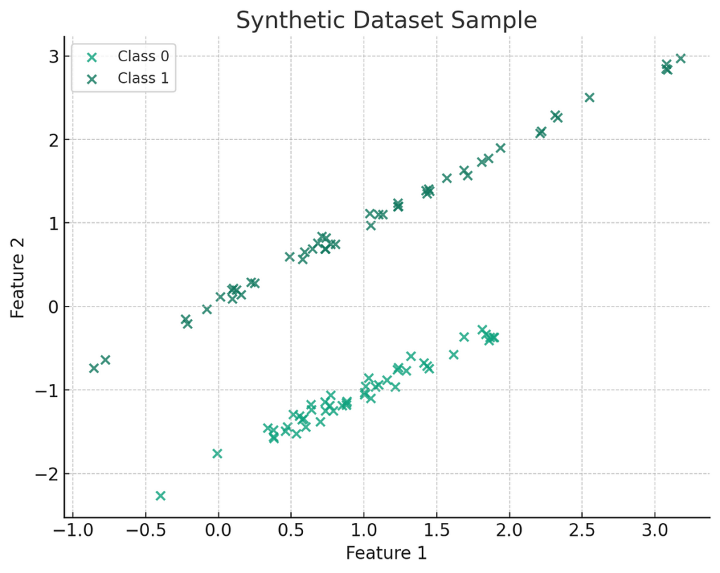
Here’s a visualization of a sample synthetic dataset with two informative features. The plot displays two classes differentiated by color. Each point represents a sample in the feature space, with the position determined by the two features. This gives you an idea of the separation between the classes and how a model might draw a decision boundary between them.
Model Loss Plot:
- Training Loss: The training loss decreases significantly and consistently over epochs, suggesting that the model learns effectively from the training data.
- Validation Loss: The validation loss decreases and starts to plateau towards the end of the epochs. This indicates that the model generalizes well to new data it wasn’t trained on. The gap between training and validation loss suggests a balance without significant overfitting.
Model Accuracy Plot:
- Training Accuracy: The training accuracy increases over time, which is expected as the model becomes better at classifying the training data.
- Validation Accuracy: The validation accuracy increases but fluctuates more than the training accuracy. This fluctuation is normal in validation curves and suggests that the model might be responding to nuances in the validation set that it hasn’t learned from the training set.
In both plots, there isn’t a wide gap between the training and validation curves, which is positive as it indicates that the model doesn’t fit the training data.
Confusion Matrix:
- The confusion matrix shows the number of true positive (TP), true negative (TN), false positive (FP), and false negative (FN) predictions.
- There are 77 true negatives, meaning the model correctly predicted the negative class 77 times.
- There are 87 true positives, meaning the model correctly predicted the positive class 87 times.
- There are 16 false positives, where the model incorrectly predicted the positive class.
- There are 20 false negatives where the model incorrectly predicted the negative class.
The model shows a reasonably balanced classification ability, with slightly more false negatives than false positives. This could be indicative of the model’s sensitivity and precision balance. In practice, the implications of FP and FN errors could be vastly different depending on the application, and it might be necessary to adjust the classification threshold or the model to reduce one type of error over the other.
Overall, the model performs well, with decent generalization from the training to the validation set and a respectable number of correct predictions. However, depending on the specific context and cost of different types of errors, you should consider strategies to balance sensitivity and specificity further.
Conclusion
Deep ensembles stand out as a potent tool in the machine learning arsenal, offering a compelling blend of accuracy, reliability, and robustness. As a practitioner, I have witnessed the transformative impact of deep ensembles across various domains, affirming their value in addressing some of the most challenging problems in machine learning. While they require thoughtful implementation and management, the benefits they provide make them an indispensable approach in the quest for superior machine learning solutions.
We’ve delved into the robust capabilities of deep-learning ensembles and their transformative potential. How do you see these strategies impacting your field of work, or what challenges do you anticipate in integrating ensemble methods into current systems? Share your insights and join the conversation to shape the future of robust AI solutions.


