
This appendix provides descriptions of the model metrics used to evaluate all of the implemented models.
Precision: Measures proportion of true positive predicted instances of all positive predictions for a given class. Formula: True Positives / (True Positives + False Positives)
Recall: Measures proportion of true positive predicted instances of all positive instances for a given class. Formula: True Positives / (True Positives + False Negatives)
F1-Score: Composite metric that uses harmonic mean of precision and recall to represent both metrics in a single number. Formula: 2 * (Precision * Recall) / (Precision + Recall)
ROC-AUC (Receiver Operating Characteristic — Area Under the Curve): Measures under ROC curve plotting true positive and false positive rate at different thresholds for classification. Serves to quantify the degree to which a model can distinguish between positive and negative instances.
Cohen’s Kappa: Ranging from -1 to 1, measuring the extent to which predicted labels and true labels agree, with values closer to 1 indicating agreement better than chance, and -1 indicating no agreement between predicted and true labels.
Formula: (Proportion of Agreement — Proportion of Expected Agreement) /
(1 — Proportion of Expected Agreement)
Recall (singles/doubles/triples): Proportion of true predicted instances of all instances for each individual class.
This appendix provides multiple graphs of all models implemented for evaluating the effect of speed on ISO, as well as visuals showing methods of data augmentation. For each model there is a confusion matrix, a dataset of metrics, a probability distribution for each class, and curves for ROC-AUC and Precision-Recall. The set of models used are as follows:
- Naive Bayes, Support Vector Classifier, Bagged Decision Trees, AdaBoost Classifier, Keras Sequential Neural Network
- Models from 1, with Principal Component Analysis and undersampling applied
- Balanced RandomForest, Weighted RandomForest (Class Weight = Balanced)
1 shows the confusion matrices for the first set of models implemented. The classes of each hit are 0 for doubles, 1 for singles, and 2 for triples. Most models predict triples as doubles, and some models predict many doubles as singles.
2 shows the metric scores evaluating the first set of models. Naive Bayes ranks worst amongst the other models in nearly every metric, while Bagged Decision Trees performs the best for all metrics. Of all models, recall for triples never exceeds five percent, and varies in terms of recall for doubles. While some models nonetheless have high ROC-AUC, the recall for each class indicates the model is not able to achieve good classification for the lowest frequency class.
3 shows the probability distributions for each class for each model. Naive Bayes and AdaBoost classifiers have many different values in their probability distributions. However, the other models have the probability of each predicted class close to 0 or 1.
4 shows ROC-AUC and Precision-Recall curves for each of the first set models implemented. In terms of ROC-AUC, Bagged Decision Trees plots the best curves, even though the AUC for triples is much lower relative to singles and doubles. All models also have poor Precision-Recall curves for doubles and triples, likely due to the lower prevalence of both classes relative to singles.
5 shows an error from the initial calculation of distance using polar r-values. Some values from Statcast projected distance were higher than the calculated distance. The inverse is supposed to happen, so for the second and third set of models, the maximum of the two is taken for each hit.
6 visualizes the training dataset augmented with 2 and 3 component PCA. In 2 components, the data is not linearly separable, with triples contained in the overlap of singles and doubles. However, separation in 3 components appears possible from different angles.
7 visualizes the training dataset augmented with 2 and 3 component PCA and undersampling. In 2 components, the data is not linearly separable, with triples contained in the space of both singles and doubles. In 3 components, the data appears more easy to separate, with some ability to tell apart each of the three classes.

8 shows the confusion matrices for the first second of models implemented. Undersampling and PCA causes overpredictions for triples, the opposite problem of the first set of models. For each model, doubles are somewhat evenly predicted across all three classes, and predictions for triples are much improved from the previous set of models.
9 shows the metric scores evaluating the second set of models. All models are more similar in terms of Precision, Recall, F-1, ROC-AUC, and Cohen’s Kappa. However, the worse performing models from the first set improved, while the better performing models got worse. Recall for singles remained high, and recall for triples sharply improved at the cost of recall for doubles.
10 shows the probability distributions for each class for each model. PCA and undersampling gives all of the models for spread out probability distributions. In addition, doubles and triples have few values with probabilities above 75–80%.
11 shows ROC-AUC and Precision-Recall curves for each of the second set models implemented. All plots exhibit less AUC relative to the first models without PCA and undersampling. The Precision-Recall curves also worsened overall for all models over all classes.
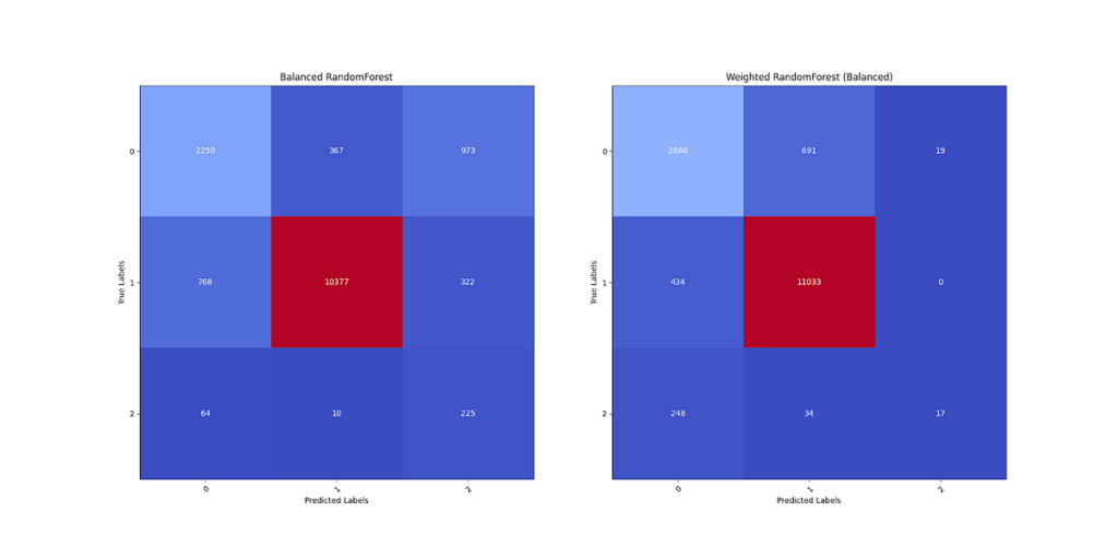
12 shows the confusion matrices for the third set of models. The Balanced RandomForest contains a similar problem from the second set of models, where triples are better predicted at the cost of predictions for singles and doubles. On the other hand, the Weighted Random Forest predicts singles and doubles apart well, but has low recall for triples. However, given the nature of the problem, the latter model was chosen due to a preference for underpredicting triples instead of overpredicting triples.
13 shows the metric scores evaluating the third set of models. The Weighted RandomForest has slight advantages to the Balanced RandomForest in terms of most metrics. However, recall for triples is as low as the first of models, while Balanced RandomForest has recall similar to the second set of models.
14 shows the probability distributions for each class for each model. Balanced RandomForest contains a similar distribution for the second set of models, while Weighted RandomForest has similar distributions to the first set of models. Overall, it is possible that probabilistic classification for hit types may be an inadequate method of classification.
15 shows ROC-AUC and Precision-Recall curves for each of the third set models implemented. Both plots exhibit the best ROC-AUC of all models implemented, differing in the AUC for doubles and triples. While the Precision-Recall AUC improved to other models, the AUC for triples was still well below that of singles and doubles.
This appendix provides visuals evaluating the Weighted RandomForest model’s predictions for ISO. Graphs include predictions of ISO plotted against true ISO values for 2022 players, residuals of predicted and true ISO, and residuals of predicted ISO given a value for sprint speed minus predicted ISO given true sprint speed.
1 is a scatterplot showing the difference between true ISO values and predicted ISO values for 2022 MLB players. In general, points fall just below the line of perfect prediction, showing a general trend of the Weighted RandomForest to underpredict ISO. Some points near the origin (below .100 ISO) show large divergence between predicted and true ISO.
2 is a residual plot showing the difference between predicted and true ISO values for 2022 MLB players. Predicted ISO is plotted on the x-axis, with the difference plotted on the y-axis. While the model tends to underpredict ISO, the average residuals of predicted ISO above true ISO appear to be much higher.
3 is a residual plot showing the difference between true ISO values and predicted ISO values given sprint speed is within 1.5 ft/sec from true sprint speed. The plot shows residuals from 200+ MLB players from 2022. Taken together, an additional 1.5 ft/sec to sprint speed results in a 0.005 increase in ISO or 1 extra base per 100 AB, on average for all players. However, the maximum and minimum residuals show a +0.020 and a -0.035 change in predicted ISO.
4 shows the residuals of predicted ISO for Giancarlo Stanton in 2022. Changes in speed provide no loss or gain in ISO.
5 shows the residuals of predicted ISO for Kyle Schwarber in 2022. Similar to Stanton, changes in speed provide little loss or gain in ISO. However, at +1.5 ft/sec, there is a gain of about 0.005.
6 shows the residuals of predicted ISO for Ronald Acuña Jr. in 2022. Increases or decreases in speed somewhat, according to the model, affect his ISO values. The range of effects on ISO range from around -0.007 to +0.008, or around 1.5 extra bases per 100 AB.
7 shows the residuals of predicted ISO for Mookie Betts in 2022. Increases in speed appear to improve his ISO more than a similar decrease in speed. Starting at +1 ft/sec of speed (which he had in past seasons with the Red Sox), he affects his ISO by at least ½ base per 100 AB. However, he experiences less of a decline if his speed were to fall further.
8 shows the residuals of predicted ISO for Alex Bregman in 2022. While Bregman used to be faster in past seasons, changes in speed affect him on a similar level as Kyle Schwarber. This would suggest that he may be a hitter who performs similar to sluggers, but is faster than the average slugger.
9 shows the residuals of predicted ISO for Starling Marte in 2022. While Marte used to be among the fastest in the game during his prime, his residuals showcase the potential effect of age. Residuals from higher sprint speed values give him an increase in ISO around 0.010. On the other hand, a further decline in speed produces little effect on ISO, about 1 extra base per 200 AB
10 shows the residuals of predicted ISO for Corbin Carroll in 2022. No effects on ISO come from increases in speed. However, there is a noticeable decrease in ISO that starts at a -0.5 ft/sec change in sprint speed. At worst, the model gives Carroll a decrease in ISO of nearly 0.010.
11 shows the residuals of predicted ISO for Bobby Witt Jr. Though Witt has similar speed to Corbin Carroll, the difference in ISO residuals from predicted ISO at true sprint speed indicate a potential effect from batted ball quality. Overall, there is little effect from changes in sprint speed: about ½ extra base per 100 AB either way.


