
Doesn’t matter whether you are Data Scientist or not, you indulge in measuring the performance or (in short) measuring the quality of things you deal with. And that’s the ultimate truth. Remember, we used to get performance cards during school days to get them signed by parents? Even today, if we visit a supermarket for grocery shopping, we do quality checks many times before we put them in our carts.
We are 360⁰ involved in quality checks or performance measures. Similar fashion, as a data scientist, check the quality of the model that you built. And that’s where all performance measurement models come into the picture. In this section, we will discuss performance measures for a classification problem.
In the Data Science life cycle, measuring the performance of the model you built comes at the end of the life cycle. Your task is to first understand the business problem, collect data as per the business problem. Once you wrap up the data collection phase, then you go with the data preparation and exploratory data analysis phase. Once we understand the data completely (regarding our problem), we build machine learning models.

Once we have done with building machine learning models next step is to verify those models or measure the performance of those models to find out good performing models for our goal. This stage is nothing but the model evaluation stage, as shown in the above figure.

In this blog post, we will focus on metrics related to classification problems. There are metrics related to regression problems as well, but that we discuss that in Part-II of this blog post. For now, we will cover below performance metrics →.
- Accuracy
- Confusion Matrix
- Precision & Recall
- F Beta
- Kohen’s Kappa
- ROC Curve
- Log Loss
Let’s start with Accuracy.
Accuracy is one of the popular metrics for evaluating classification models. In classification problems, we calculate accuracy in two ways →.


Problems with Accuracy Measure
There are issues with accuracy measures and hence it is not a widely used performance metric in data science. Let’s discuss the problems faced by accuracy measures.
Problem 1 → Imbalanced Data
Accuracy is a good performance measure when you have perfectly balanced data. But that’s not the reality always. You may or may not have perfectly or somewhat balanced data to accept the accuracy as the performance metric.

Let’s say, you have got a classification dataset about Xi and the class label of that dataset is (Yi) “Has cancer” or “No Cancer”. Basically, you are trying to classify whether a patient will be diagnosed with cancer or not?. Let’s look at the nitty-gritty details of the dataset.

If your dataset is above mentioned one then given query point (Xq), the model will classify it to the “Negative” category with an accuracy of 90%. With such a faulty model, we get pretty good accuracy. This is a concerning thing regards to an accuracy performance metric.
When there is a case of imbalanced data, never use accuracy as a model performance trait.
Problem 2 → Predicted Class Label Vs Probability Score
Many algorithms can provide probability scores of their prediction as well as predict class labels. Let’s use this functionality of models to illustrate this concept.
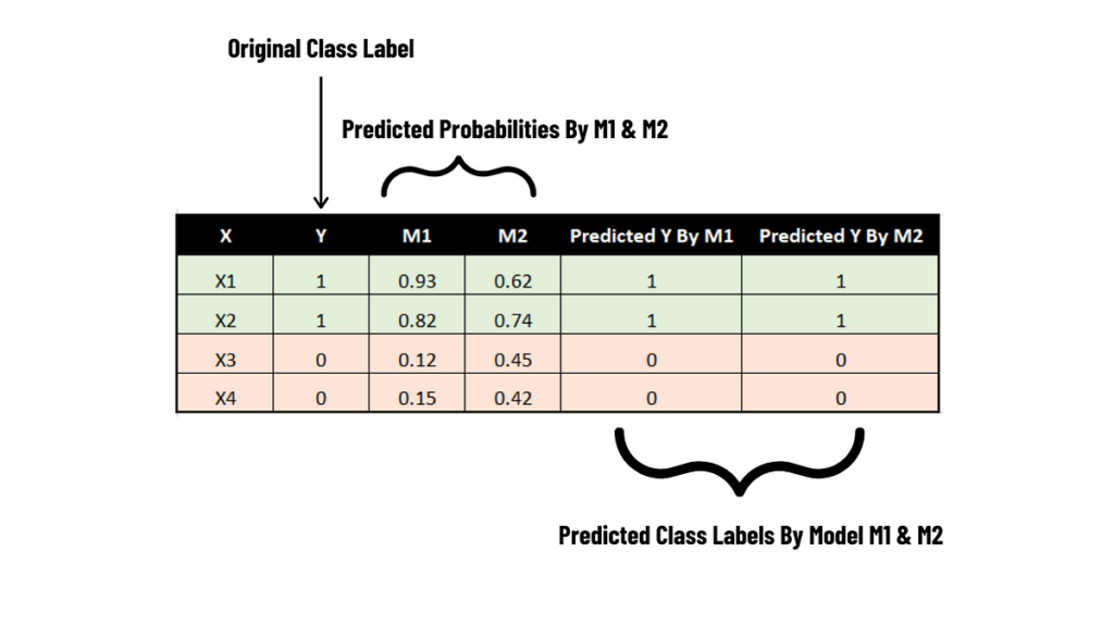
Let’s say you have a dataset with two features is X & Y. (Here we are predicting Y based on variable X). Let’s use two models (Let me call them M1 & M2) to do the predictions.

Observations →
- Model M1 & M2 return probability scores & also, depending upon the probability score, we have labelled them in the above problem.
- For X1, the original class label is 1. With the help of M1 (P (Y=1|X1) we got the probability of 0.93 and with M2, we got the probability of 0.62. Both model labelled Y as 1 due to (P (Y=1|X1) > 0.50.
- For X2, the original class label is 1. With the help of M1 (P (Y=1|X2) we got the probability of 0.82 and with M2, we got the probability of 0.74. Both model labelled Y as 1 due to (P (Y=1|X2) > 0.50.
- For X3, the original class label is 0. With the help of M1 (P (Y=1|X3) we got the probability of 0.12 and with M2, we got the probability of 0.45. Both the model labeled Y as 0 due to (P (Y=1|X3) < 0.50.
- For X4, the original class label is 0. With the help of M1 (P (Y=1|X4) we got the probability of 0.15 and with M2, we got the probability of 0.42. Both the model labeled Y as 0 due to (P (Y=1|X4) < 0.50.
Models M1 and M2 predicted class labels accurately as predicted and actual class labels are the same in all situations.
By observing the table, we can conclude that model M1 is better performing model than model M2 by looking at their probability score. Unfortunately, performance measures like accuracy cannot use the probability score, it can only use the class labels. Model M1 and M2 has same accuracy, but looking at probability score, we know M1 is better than M2.
There is another classification performance metric known as the confusion matrix used widely in classification problems in statistics and machine learning. We define the confusion matrix as →.
In machine learning or in statistical classification, a table of confusion (sometimes also called as Error Matrix) is a table with two rows and two columns shows the performance of the classification algorithm by comparing ‘Actual Vs Predicted Class Labels’.
When we have a binary classification problem, then the grid of the confusion matrix is 2×2. (Confusion Matrix is mostly used in Binary Classification Problems)

Like Accuracy, the Confusion Matrix does not process the Probability Score!
If your model is sensible, all principle diagonal elements should be high and off-diagonal elements should be low.

Understanding TN TP FN FP
A confusion matrix is built with the help of the following concepts →
- TN (True Negative),
- TP (True Positive),
- FN (False Negative),
- FP (False Positive)

Now, let’s understand each of these concepts briefly.
True Positive (TP)
- The model has predicted positive and actual is positive too.
- Ex → Model has predicted a woman is pregnant, and she actually is.
True Negative (TN)
- The model has predicted negative, and actual is negative too.
- Ex → Model has predicted that a man is not pregnant, and he actually isn’t.
False Positive (FP)
- The model has predicted positive but the actual is negative.
- This is nothing but a Type-I error.
- Ex → Model has predicted that a man is pregnant but actually he isn’t.
False Negative (FN)
- The model has predicted negative but actually is positive.
- This is the case of Type-II error.
- Ex → Model has predicted woman is not pregnant, but she actually is.
By using the above information, we can calculate the list of rates from the confusion matrix for a binary classifier. Let’s understand these rates now.
Various Performance Metrics Derived From Confusion Matrix
Let’s understand the various performance metrics that can be calculated from the confusion matrix itself with the help of a toy example.

Accuracy
- Overall, how often is the classifier is correct?
- Accuracy = (TN + TP) / (TN + TP + FN + FP) = 175 / 200 = 0.87
Misclassification Rate
- Overall, how often your classifier is wrong?
- Misclassification Rate = (FN + FP) / (TN + TP + FN + FP) = 25/200 = 0.125
True Positive Rate (TPR)
- When it’s actually “Yes”, how often does your model predict “Yes”.
- This is also known as “Sensitivity” or “Recall”
- TPR = TP / P = TP / (FN + TP) = 100 / 105 = 0.95
- It is equivalent to 1-FNR
True Negative Rate (TNR)
- When it’s actually “No”, how often does your model predict “No”?
- It is also known as “Specificity” or “Selectivity”
- TNR = TN / N = TN / (TN + FP) = 75 / 95 = 0.78
- It is equivalent to 1-FPR
False Positive Rate (FPR)
- When it’s actually “No”, how often does your model predict “Yes”?
- It is also known as “Type-I error” or “Fall-out”
- FPR = FP / N = FP / (TN + FP) = 20 / 95 = 0.21
- It is equivalent to 1-TNR
False Negative Rate (FNR)
- When it’s actually “Yes”, how often does your model predict “No”?
- It is also known as “Type-II error” or “Miss Rate”.
- FNR = FN / P = FN / (FN + TP) = 5 / 105 = 0.04
- It is equivalent to 1-TPR
Balanced Accuracy (BA)
- It is a simple arithmetic mean of “Sensitivity” and “Specificity”.
- BA = TPR + TNR / 2 = 0.95 + 0.78 / 2 = 0.86
Your Model will be good, if TPR & TNR is high and FNR & FPR is low. In simple words, all the principle diagonal elements must be high and off-diagonal element must be low.
These are the metrics also calculated from the confusion matrix only. The reason I have kept them separate as topics is that they are highly important metrics in binary classification problems.
Let’s discuss them now.
Precision
- Precision is the concept is taken from Information Retrieval and Pattern Recognition.
Precision, which is also known as Positive Predictive Value (PPV) defined as →
It is a fraction or percentage of relevant instances among the retrieved instances.
- In our binary classification problem, we can say precision is, “All the points that the model declared or predicted to be positive, what % of them are actually positive?”
- Precision is actually the ratio of True Positive (TP) to True Positive & False Positive.

Example →
For fishing, you throw a fishing net into the river/pond/ocean. After some time you pull it back considering that you have trapped enough fish. But what you get is some fish and some plastic (Garbage). So in this case your precision would be →
“All the stuff that you caught, what % them are actually fish?”
Recall
- The recall is nothing but the True Positive Rate (TPR) is defined as →
It is fraction, or percentage, of relevant instances that were retrieved from total relevant instances.
- In binary classification lingo, we can say, “When it’s actually ‘Yes’, how often does your model predict ‘Yes’?
- It is also known as “Sensitivity”.

Example →
In the above fishing example, the recall would be →
“Out of all the fish in the ocean, what % of fish did you catch?”
Precision & Recall are very much important when you care about positive class in classification problems.

Example: Medical Diagnosis for a Disease
Imagine you have developed a machine learning model to diagnose a rare but serious disease, where:
- “Positive” means the model predicts the disease is present.
- “Negative” means the model predicts the disease is not present.
Now, consider the following outcomes from testing 1000 patients:
- True Positives (TP): 80 patients truly have the disease, and the model correctly diagnoses them as having the disease.
- False Positives (FP): 20 patients do not have the disease, but the model incorrectly diagnoses them as having the disease.
- True Negatives (TN): 880 patients truly do not have the disease, and the model correctly identifies them as not having the disease.
- False Negatives (FN): 20 patients have the disease, but the model incorrectly identifies them as not having the disease.
Precision (Quality of Positive Predictions):
In our example, precision represents how accurate the model is when it predicts that a patient has the disease:

So, the precision of your model is 0.80 or 80%. This means that when the model predicts the disease, it is correct 80% of the time.
Recall (Capturing Actual Positives):
Recall, on the other hand, represents how well the model can identify patients who actually have the disease:

So, the recall of your model is also 0.80 or 80%. This means that out of all the patients who truly have the disease, the model correctly identifies 80% of them.
Interpretation and Use-Case:
- Precision: If the disease is one where the treatment has severe side effects, you might prioritize precision. This is because you want to be very sure that patients diagnosed with the disease actually have it before subjecting them to the treatment. In our example, a precision of 80% is fairly high, which is good if the treatment has significant risks.
- Recall: If the disease is extremely dangerous or infectious, you might prioritize recall. This is because you want to ensure that nearly all individuals who have the disease are identified, even if that means some false positives. In our example, a recall of 80% means that we’re capturing a good proportion of actual cases, but we might want to improve this if the disease is severe and missing a case could be deadly.
In the last topic, we’ve discussed the most important metrics in classification that is Precision & Recall. If you could remember, we have stated also that →
- When we care more about the False Positive (FP) than False Negative (FN), we use Precision.
- When we care more about the False Negative (FN) than False Positive (FP), we use Recall.
But what if in the situation, you need both metrics at the same time? If yes, instead of stating each of these metrics separately, Is there any way to combine these two metrics? → Yes, and the answer lies in the F-βeta concept. Let’s discuss it.

With F-βeta, a usually most important task is to select the value of βeta. Let’s take various βeta values and discuss various cases.
When βeta = 1
- When we have βeta = 1 then the above F-βeta equation becomes F1-Score.
- F1 Score is nothing but the Harmonic Mean between Precision & Recall.
- If Precision & Recall both are equally important in the problem statement or aim, we use βeta = 1.
When βeta = 0.5
- In some cases, False Positive (FP) has more impact than False Negative (FN) then we reduce the βeta value to 0.5
- It is also known as the F0.5 Score.
- Use βeta = 0.5 whenever a Type I error is more important than Type II.
When βeta = 2
- In some cases, False Negative (FN) has more impact than False Positive (FP) then we increase our βeta value to 2.
- It is known as the F2 Score.
- Remember we use βeta value > 1 when type II error has more impact than type I error on the model.


