
Introduction
Let’s say that you have collected some information on kids living in your neighbourhood –
You really want to figure out what makes someone go outdoors and play, based on a few conditions about the person or the environment. What you would like even better is to be able to create some sort of a program, a model, that could predict with acceptable accuracy for kids other than the ones from whom you have collected the data.
To do this, you would need a classifier that could take in this information, process it, and be able to pop out a ‘Yes’ or ‘No’ whenever new information is provided. And do this, you could use a Decision Tree Classifier.
One of the more popular algorithms used widely in the field of machine learning is the Decision Tree. It can be used to solve two kinds of problems-
- Classification — you label the data out of two or more classes based on the input parameters in the data. When there are only two classes, it is also called ‘binary classification’.
- Regression — instead of discrete class labels, you predict a continuous value variable, such as salary or age.
In this blog, I will be focusing on the Decision Tree Classifier. And as you may have noticed, our small dataset requires us to classify the data into two labels based on whether or not the person decides to go out and play.
Terminology and How it works

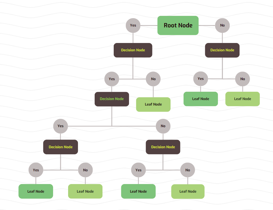
The Decision Tree works by creating various branches, nodes, and leaves.
Each node will ask a question that will segregate the data coming into it into two (or more, but generally two) ‘childern nodes’.These children nodes are connected to the ‘parent node’ by branches.
When a node doesn’t split further, it is termed as a ‘leaf node’.
The highest node is the ‘root node’, which contains all the data you have collected. You can imagine this as an inverted tree — with the root at the top and the leaves at the bottom.
‘Attribute’ refers to each column of data.
At each node, we will consider one or more attributes of the data and split the incoming data based on certain values of those attributes.
How to decide which attributes to split on?
To make our very own simple Decision Tree, we will put just one attribute in each node.
For the root node, we can select one of three attributes — whether or not it is raining, whether or not the kid likes cats, and the kid’s age. How do we decide which one is best?
Thankfully, we have two important mathematically sound techniques that will help us do just that.
- Gini Index / Impurity
It is used to garner the possibilty of randomly selected sample being wrongly classified by a node.
Let’s segregate our data based on the attribute ‘Is raining’ in the root node.

The number below the ‘Yes’ and ‘No’ represents the number of kids.
The formula for calculating Gini Index is –

Here, pⱼ is the probablity of a particular datapoint belonging to a class.
Gini index for our node = 1 — (probability of ‘Yes’)² — (probability of ‘No’)²
For the left node, GI = 1 — (1/4)² — (3/4)² = 0.375
For the right node, GI = 1 — (3/3)² — (0/3)² = 0
Gini index lies between 0 and 0.5. The lower it is, the ‘purer’ the data in that node is, i.e., the more likely it is that the data belongs to a single class.
In case of the right node, all the datapoints had ‘Yes’ as an answer to the question of whether or not they would play outside. This gave the node a perfect Gini index of 0.
In order to calculate the Gini index of the parent node, in this case the root node, we will take the weighted mean of the Gini indexes of the children nodes, with the weights being the number of datapoints in each node.
For the root node, GI = 0.375 * (4/7) + 0 * (3/7) = 0.214
Hence, the GI corresponding to the attribute ‘Is raining’ is 0.214.
Similarly, we can calculate the GI for the other attributes.

Left node GI = 1 — (2/4)² — (2/4)² = 0.5
Right node GI = 1 — (2/3)² — (1/3)² = 0.444
Root node GI = 0.5 * (4/7) + 0.444 * (3/7) = 0.476
Calculating the GI for the age attribute is trickier. It cannot be separated into clear ‘Yes’ and ‘No’ answers. In case of such numerical data, we will decide on a value x and create two categories for datapoints, where –
The age category has already been arranged in ascending order for convenience. We can choose x to be the averages of two consecutive ages. Hence, x will take the values {7.5, 9.5, 11, 12.5, 14, 16}. We will calculate the GI for each value of x. I am skipping the repetitive calculations; here are the GIs –
Remember, the Gini index measures the impurity of the data. We want it to be as low as possible. Among the values of x, x = 16 has the lowest GI. However, the attribute ‘Is raining’ has the lowest GI among all possible attrbutes at 0.214.
Hence, we will select this attribute for the root node.
2. Information gain
Before delving into Information gain, we will define another term called ‘Entropy’. Just like GI, it is also a measure of the impurity of a node.

Here, pᵢ is the probablity of a particular datapoint belonging to a class — the same as before. E(S) lies between 0 and 1.
Let’s find the entropies of all the nodes in the ‘Is raining’ split.
E(root node) = – (4/7) * log₂(4/7) – (3/7) * log₂(3/7) = 0.985
E(left node) = – (1/4) * log₂(1/4) — (3/4) * log₂(3/4) = 0.811
E(right node) = – (3/3) * log₂(3/3) — (0/3) * log₂(0/3) = 0
Now, we can calculate information gain. It is defined as the sum of weighted entropies of the children nodes subtracted from the entropy of the parent node. Mathematically, if A is the attribute that we are calculating for, S is the data set, and v represents the classes –

Information gain for ‘Is raining’ will be –
IG = E(root node) – (4/7) * E(left node) – (3/7) * E(right node)
IG = 0.985 – (4/7) * 0.811 – (3/7) * 0 = 0.522
The higher the IG, the more information is gained after splitting. Now, let’s calculate the IG for the attribute ‘Likes cats’.
E(root node) = — (4/7) * log₂(4/7) — (3/7) * log₂(3/7) = 0.985
E(left node) = — (2/4) * log₂(2/4) — (2/4) * log₂(2/4) = 1
E(right node) = — (2/3) * log₂(2/3) — (1/3) * log₂(1/3) = 0.918
IG = 0.985 – (4/7) * 0.5 – (3/7) * 0.918 = 0.020
Clearly, this attribute is terrible for prediction.
We can similarly calculate the IGs for the numerical attribute age.
Both methods of calculating impurity have their pros and cons. Gini index is will-suited for binary classification, because it is computationally more efficient. On the other hand, Information gain takes the lead in an unbalanced dataset, or in a dataset with multiple classes.
When to stop adding node?
We can split the nodes based on either of the above two techniques. But when do we stop adding decision nodes and terminate with leaf nodes? Ideally, we will end up with leaf nodes where all the data belongs to one class. The node will then simply predict that class as its output.
This is often practically infeasible. If we do end up with such nodes, our trees tend to be very deep, take a long time to train, and cause issues such as overfitting. This implies that the classifier does a good job predicting on the training dataset, but performs poorly on the testing dataset.
We could also leave the node impure, with the data belonging to more than one class. The output will then be decided based on the majority class.
Let’s create decision nodes in our incomplete tree.
We will have to calculate either Gini index or Information gain for all attributes at both nodes. Since the former is better for binary classification, we will go with Gini index.
Left node –
In this case, we don’t even need to calculate Gini index for each attribute. We can simply use age as an attribute, splitting the data based on age > 7.5 and age < 7.5
Right node –
This one doesn’t require any more decision nodes. We can convert the right node into a leaf node
Our final decision tree looks like –

Hooray! We have completed building our very own tree by training it on our dataset! Now, when given fresh information about other kids, we should be able to predict whether or not they will play outside.
You will notice that we have ignored the attribute ‘Likes cats’. It simply was not a good predictor of being or not being outdoors, so we can drop it.
Let’s take a kid with the following attributes :
Is raining : Yes
Likes cats : No
Age : 8

Our classifier predicts that the kid won’t go out to play.
There is a problem with this prediction – we have just one datapoint where it’s raining and the kid goes out to play. We cannot be sure whether it will be reliably true for other kids based on so little information. It is possible that our decision tree is overfitting – it has tried to fit itself to the training data too strongly, making it unreliable for unseen data. This is a common problem we face in training Decision Tree models.
One way to fix this would be to simply convert the decision node that splits based on age into a leaf node. This would make the node impure — we would have 3 ‘Yes’ and 1 ‘No’. The output from the leaf will be ‘Yes’, which is 75% accurate, but it isn’t affected by a single datapoint. Our tree will now look like –

This is possibly better suited for predictions on unseen data. To quantify which model is better, we will have to test it on unseen data.
In our simple example, it was easy to determine when to stop adding decision nodes. In a real-life scenario, we will have thousands of rows of data and tens of columns of attrtibutes. Our tree will be very complex, and deciding when to turn a node into a leaf node becomes a very important task.
Let’s discuss some hyperparameters that Decision Trees have, and how we can reduce overfitting and make decisions on splitting.
Hyperparameters
Decision trees make few assumptions about the training data. If the model is not constrained, it will heavily conform to the training set, resulting in overfitting.
There are internal parameters in every ML model that are learnt based on the training dataset. These are responsible for making predictions. They vary with the data fed and are out of our control.
There are some parameters called ‘hyperparameters’ which control the learning process of a model. We can choose hyperparameters for a model before the training process starts. They cannot be varied during training, and hence can be considered as external parameters.
When faced with overfitting, hyperparameter tuning is a crucial step in resolving this issue. It is essential to get a usable model.
We will focus on these important hyperparameters of a Decision Tree –
- criterion : This helps in choosing which attributes to split a node on. We can choose criteria like Gini index and Entropy. Which one to choose depends on the type of data, number of classes, and computing resources available.
- splitter : This is the strategy used for splitting nodes. We can choose either ‘best’, or ‘random’. In case of ‘best’, it will use the criterion to decide the best attribute, while the attribute will be selected at random in case of ‘random’.
- max_depth : This is defined as the maximum depth of the tree, or the maximum number of nodes from the root node to a leaf node. By default, this value is unconstrained — the model can be as deep as possible. In our little example, we saw how this could result in the model overfitting on the training data. Reducing the max_depth is a good method to reduce overfitting.
- min_samples_split : A node will be split only if the number of datapoints in it is greater than min_samples_split. If the value is, say, 5, then a node won’t be split if it has 5 or lesser datapoints. The node will become a leaf node and the output will be decided based on the majority class.
- min_samples_leaf : This specifies the minimum number of datapoints that must be present in a leaf node. If this value is 3, and a node has 5 datapoints, then it can’t be split any more. In our example, the decision node ‘Age < 7.5’ wouldn’t be formed if the value was greater than one — a leaf node would be unable to contain just a single datapoint.
- max_features : The number of features that a decision node takes into consideration is affected by this number. We can have a decision node only consider a fraction, or the square root, or log₂ of the total number of features.
Varying the last four hyperparameters has the added effect of reducing the complexity of the model and decreasing training time. Changing them will decrease the accuracy of the model on the training dataset, but will hopefully increase the accuracy for unseen data.
How do we decide which set of parameters is best for the model? One which does not overfit, and also manages an acceptable accuracy on testing data?
We can use something called ‘Grid Search’, which takes several parameters for each hyperparameter, and tries every combination for train a model. It will return the parameters that give the best accuracy.
We also use something called ‘Cross-validation’, which divides the training dataset into several smaller subsets. The model is trained on all but one subset, and is then tested on the remaining subset. All subsets form the testing set one by one. This gives a better prediction of accuracy of the model. k-fold cross-validation implies that the training dataset is divided into k subsets.

These two are used in conjunction for various ML models, not just Decision Trees.
Advantages and Disadvantages of Decision Trees
Now that we know all about how Decision trees are built, we are ready to figure out what it can offer, and what are its drawbacks –
- It works well with both numerical and categorical data. We do not need to convert the categorical columns into numerical columns.
- The numerical data does not need to be scaled.
- Missing / incomplete data does not affect the model too much. These few steps mean that we can forgo a decent portion of data processing. This makes the model beginner-friendly.
- The model tends to overfit a lot. Hyperparameter tuning is necessary to create an actually usable model.
- The model takes a fairly large chunk of time and computing resources in training.
- At each node, the model decides the attributes on which to split based on lowest impurity, and does not consider how it may affect the next few splittings. This is the reason why the algorithm is considered to be a greedy algorithm. The final tree created may not be the most optimal. This is where the hyperparameter ‘splitter’ may come into play. By randomly deciding the splitting attribute, it could chance upon a more optimal model.
- It works better on classification problems than on regression problems.
Training and testing a Decision Tree model
Let’s take an actual dataset and make an ML model.
Not all the code that was written for the model is shown here — only the important portions are highlighted. To view the entire code, here’s the link to the Kaggle notebook where the code is saved.
import pandas as pd
import numpy as np
from matplotlib import pyplot as plt
import seaborn as sns
import plotly.express as pxpd.set_option('display.max_columns', None)
sns.set_style('darkgrid')
from sklearn.tree import plot_tree
from sklearn.tree import DecisionTreeClassifier
from sklearn.model_selection import train_test_split
from sklearn.metrics import accuracy_score
from sklearn.metrics import confusion_matrix
from sklearn.model_selection import GridSearchCV
df = pd.read_csv("/kaggle/input/employee-dataset/Employee.csv")
To start with, we import some necessary libraries. Pandas and NumPy are essential libraries for any ML model. Scikit-learn is a ML library that contains various models including Decision Trees. We also import several scoring metrics and plotting features.
categorical_cols = ['Education', 'City', 'Gender', 'EverBenched']
df = pd.get_dummies(df, columns = categorical_cols)df['Education_Bachelors'].replace([True, False], [0, 1], inplace = True)
df['Education_Masters'].replace([True, False], [0, 1], inplace = True)
df['Education_PHD'].replace([True, False], [0, 1], inplace = True)
df['City_Bangalore'].replace([True, False], [0, 1], inplace = True)
df['City_New Delhi'].replace([True, False], [0, 1], inplace = True)
df['City_Pune'].replace([True, False], [0, 1], inplace = True)
df['Gender_Female'].replace([True, False], [0, 1], inplace = True)
df['Gender_Male'].replace([True, False], [0, 1], inplace = True)
df['EverBenched_No'].replace([True, False], [0, 1], inplace = True)
df['EverBenched_Yes'].replace([True, False], [0, 1], inplace = True)
We convert all categorical data into numerical data. Scikit-learn cannot handle categorical data — it must be converted.
train_df, test_df = train_test_split(df, test_size = 0.3, stratify = df['LeaveOrNot'])y_train = train_df['LeaveOrNot'].copy()
X_train = train_df.drop(['LeaveOrNot'], axis=1)
y_test = test_df['LeaveOrNot'].copy()
X_test = test_df.drop(['LeaveOrNot'], axis=1)
We split the dataset into training and testing datasets with a 70/30 split.
We also separate the inputs and targets into different dataframes.
from imblearn.over_sampling import SMOTEsm = SMOTE(random_state=42)
X_train, y_train = sm.fit_resample(X_train, y_train)
The number of employees that left the company make a minor portion of the entire dataset. Training on this unbalanced dataset will cause the model to perform poorly with unseen data when predicting attrition. Hence, we have balanced the dataset.
dtree = DecisionTreeClassifier()
dtree.fit(X_train, y_train)
We now train a simple Decision Tree model without any hyperparameter tuning.

The model performs fairly good on the testing dataset.
We will now use grid search to look for a better set of parameters.
param_grid = {
'criterion': ['gini', 'entropy'],
'max_depth': [None, 2, 3, 5, 8, 10],
'min_samples_split': [2, 3, 4],
'min_samples_leaf': [1, 2, 3]
}gdt = DecisionTreeClassifier()
grid_search = GridSearchCV(estimator=gdt, param_grid=param_grid, cv=5, scoring='accuracy')
grid_search.fit(X_train, y_train)
best_params = grid_search.best_params_
print("Best parameters: ", best_params)
best_gdt = DecisionTreeClassifier(**best_params, random_state=42)
best_gdt.fit(X_train, y_train)

The model is still not very accurate in cases of attrition, but the overall accuracy has increased. We can try more hyperparameters, and different values for existing hyperparameters to try and get an even better model.
Bibliography and Resourcess


