
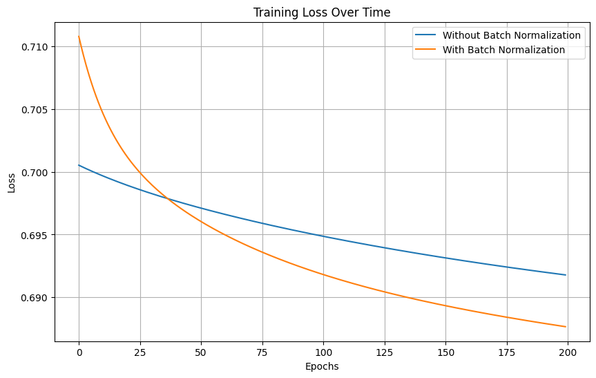
TL;DR: Models converge faster and to a lower when using batch normalization.
Batch Normalization is a method used to make artificial neural networks faster and more stable through normalization of the input layer by re-centering and re-scaling. It was proposed by Sergey Ioffe and Christian Szegedy in their 2015 paper, “Batch Normalization: Accelerating Deep Network Training by Reducing Internal Covariate Shift”.
3 examples below:
- 1 minimal example using pure pytorch on random data
- A more thorough example for different model sizes looking at both train and val loss
- An example on MNIST
Spoiler: Batch normalization converged faster every time and achieved better loss.

import torch
import torch.nn as nn
import torch.optim as optim
import matplotlib.pyplot as plt# Set seed for reproducibility
torch.manual_seed(0)
# Create dummy data for binary classification
input_dim = 10
n_samples = 1000
X = torch.randn(n_samples, input_dim)
y = torch.randint(0, 2, (n_samples,))
# Define the number of epochs and learning rate
epochs = 200
lr = 0.01
# Define a simple model without batch normalization
class ModelWithoutBN(nn.Module):
def __init__(self):
super(ModelWithoutBN, self).__init__()
self.layer = nn.Sequential(
nn.Linear(input_dim, 100),
nn.ReLU(),
nn.Linear(100, 1),
)
def forward(self, x):
return self.layer(x)
# Define a simple model with batch normalization
class ModelWithBN(nn.Module):
def __init__(self):
super(ModelWithBN, self).__init__()
self.layer = nn.Sequential(
nn.Linear(input_dim, 100),
nn.BatchNorm1d(100),
nn.ReLU(),
nn.Linear(100, 1),
)
def forward(self, x):
return self.layer(x)
# Initialize the models
model_without_bn = ModelWithoutBN()
model_with_bn = ModelWithBN()
# Define the loss function and the optimizers
criterion = nn.BCEWithLogitsLoss()
optimizer_without_bn = optim.SGD(model_without_bn.parameters(), lr=lr)
optimizer_with_bn = optim.SGD(model_with_bn.parameters(), lr=lr)
# Placeholders for losses
losses_without_bn = []
losses_with_bn = []
# Training loop
for epoch in range(epochs):
for model, optimizer, losses in [(model_without_bn, optimizer_without_bn, losses_without_bn),
(model_with_bn, optimizer_with_bn, losses_with_bn)]:
optimizer.zero_grad()
outputs = model(X).view(-1)
loss = criterion(outputs, y.float())
loss.backward()
optimizer.step()
losses.append(loss.item())
# Plot the losses
plt.figure(figsize=(10, 6))
plt.plot(losses_without_bn, label='Without Batch Normalization')
plt.plot(losses_with_bn, label='With Batch Normalization')
plt.xlabel('Epochs')
plt.ylabel('Loss')
plt.title('Training Loss Over Time')
plt.legend()
plt.grid(True)
plt.show()
Let’s do a more thorough test with different model depth and width, using some data that have a pattern, looking at both the validation and train loss:

import torch
import torch.optim as optim
import matplotlib.pyplot as plt
from matplotlib.lines import Line2D
import torch.nn as nn# Set seed for reproducibility
torch.manual_seed(0)
# Define the characteristics of the data
input_dim = 10
n_samples = 1000
# Define the depths and widths to benchmark
depths = [2, 10]
widths = [100, 500]
# Define the number of epochs and learning rate
epochs = 200
lr = 0.01
# Define a function to create a model with a specified depth and width
def create_model(depth, width, batch_norm):
layers = []
for i in range(depth):
if i == 0:
layers.append(nn.Linear(input_dim, width))
else:
layers.append(nn.Linear(width, width))
if batch_norm:
layers.append(nn.BatchNorm1d(width))
layers.append(nn.ReLU())
layers.append(nn.Linear(width, 1))
return nn.Sequential(*layers)
# Define the loss function and the optimizers
criterion = nn.BCEWithLogitsLoss()
# Create dummy data for binary classification with a pattern
X_train = torch.randn(n_samples, input_dim)
y_train = (X_train.sum(dim=1) > 0).float()
# Create validation data with the same pattern
X_val = torch.randn(n_samples, input_dim)
y_val = (X_val.sum(dim=1) > 0).float()
# Initialize the models, optimizers, and loss placeholders
results = []
for depth in depths:
for width in widths:
for bn in [False, True]:
key = f'depth={depth}, width={width}, BN={bn}'
model = create_model(depth, width, bn)
optimizer = optim.SGD(model.parameters(), lr=lr)
loss_train = []
loss_val = []
results.append({
'key': key,
'model': model,
'optimizer': optimizer,
'loss_train': loss_train,
'loss_val': loss_val
})
# Training loop
for epoch in range(epochs):
for result in results:
optimizer = result['optimizer']
model = result['model']
optimizer.zero_grad()
outputs_train = model(X_train).view(-1)
loss_train = criterion(outputs_train, y_train.float())
loss_train.backward()
optimizer.step()
result['loss_train'].append(loss_train.item())
# Calculate validation loss
with torch.no_grad():
outputs_val = model(X_val).view(-1)
loss_val = criterion(outputs_val, y_val.float())
result['loss_val'].append(loss_val.item())
# Create subplots for training and validation losses
fig, axs = plt.subplots(2, 1, figsize=(14, 10))
# Line styles and labels for models with and without batch normalization
styles = ['-', '--']
bn_labels = ['Without BN', 'With BN']
# Define labels for depths and widths
depth_width_labels = [f'depth={depth}, width={width}' for depth in depths for width in widths]
# Colors for each depth and width combination
colors = ['blue', 'green', 'red', 'purple']
# Plot the training losses
for i, result in enumerate(results):
linestyle = styles[int('BN=True' in result['key'])]
color = colors[i // 2]
axs[0].plot(result['loss_train'], linestyle=linestyle, color=color)
# Plot the validation losses
for i, result in enumerate(results):
linestyle = styles[int('BN=True' in result['key'])]
color = colors[i // 2]
axs[1].plot(result['loss_val'], linestyle=linestyle, color=color)
custom_lines = [Line2D([0], [0], color="black", linestyle=styles[0]),
Line2D([0], [0], color="black", linestyle=styles[1])] +
[Line2D([0], [0], color=colors[i], linestyle='-') for i in range(len(depth_width_labels))]
# Set labels and titles
for ax, title in zip(axs, ['Training Loss Over Time', 'Validation Loss Over Time']):
ax.set_xlabel('Epochs')
ax.set_ylabel('Loss')
ax.set_title(title)
ax.grid(True)
# Add the legend
axs[0].legend(custom_lines, bn_labels + depth_width_labels)
# Adjust the layout
plt.tight_layout()
plt.show()
Let’s do that on a real dataset, the one and only MNIST (a subset of 10k examples for the train, 1k for the val). This code runs on google colab without GPU 🙂
import pytorch_lightning as pl
import torch
from torch.nn import functional as F
from torch.utils.data import DataLoader, random_split, Subset
from torchvision.datasets import MNIST
from torchvision import transforms
import os
from pytorch_lightning.callbacks.early_stopping import EarlyStopping
from pytorch_lightning.loggers import CSVLogger# Set seed for reproducibility
pl.seed_everything(0)
# Prepare MNIST dataset
dataset = MNIST(os.getcwd(), download=True, transform=transforms.ToTensor())
indices = torch.arange(0, 11000)
dataset = Subset(dataset, indices)
train, val = random_split(dataset, [10000, 1000])
train_loader = DataLoader(train, batch_size=64)
val_loader = DataLoader(val, batch_size=64)
class LitModel(pl.LightningModule):
def __init__(self, batch_normalization=False):
super().__init__()
# Simple MLP
if batch_normalization:
self.layer = torch.nn.Sequential(
torch.nn.Linear(28 * 28, 128),
torch.nn.BatchNorm1d(128),
torch.nn.ReLU(),
torch.nn.Linear(128, 256),
torch.nn.BatchNorm1d(256),
torch.nn.ReLU(),
torch.nn.Linear(256, 10),
)
else:
self.layer = torch.nn.Sequential(
torch.nn.Linear(28 * 28, 128),
torch.nn.ReLU(),
torch.nn.Linear(128, 256),
torch.nn.ReLU(),
torch.nn.Linear(256, 10),
)
def forward(self, x):
# flatten image input
x = x.view(x.size(0), -1)
return self.layer(x)
def training_step(self, batch, batch_idx):
x, y = batch
y_hat = self(x)
loss = F.cross_entropy(y_hat, y)
self.log(
"train_loss", loss, on_step=True, on_epoch=True, prog_bar=True, logger=True
)
return loss
def validation_step(self, batch, batch_idx):
x, y = batch
y_hat = self(x)
loss = F.cross_entropy(y_hat, y)
self.log("val_loss", loss, prog_bar=True)
def configure_optimizers(self):
return torch.optim.Adam(self.parameters(), lr=0.001)
def train_model(model, batch_normalization, name):
# Train the model
early_stop_callback = EarlyStopping(
monitor="val_loss", patience=3, verbose=True, mode="min"
)
csv_logger = CSVLogger("logs_folder", name=name)
trainer = pl.Trainer(
max_epochs=200,
accelerator="cpu",
callbacks=[early_stop_callback],
logger=csv_logger,
)
trainer.fit(model, train_loader, val_loader)
# Train model without batch normalization
model_without_bn = LitModel(batch_normalization=False)
train_model(model_without_bn, False, "without_batch_norm")
# Train model with batch normalization
model_with_bn = LitModel(batch_normalization=True)
train_model(model_with_bn, True, "with_batch_norm")
Visualize the loss over time:
import pandas as pd
import matplotlib.pyplot as plt# Load the metrics from the CSV file into a pandas DataFrame
df_without_bn = pd.read_csv('logs_folder/without_batch_norm/version_0/metrics.csv')
df_with_bn = pd.read_csv('logs_folder/with_batch_norm/version_0/metrics.csv')
# Forward fill NaN values in the 'val_loss' and 'train_loss_epoch' columns
df_without_bn[['val_loss', 'train_loss_epoch']] = df_without_bn[['val_loss', 'train_loss_epoch']].fillna(method='ffill')
df_with_bn[['val_loss', 'train_loss_epoch']] = df_with_bn[['val_loss', 'train_loss_epoch']].fillna(method='ffill')
# Plot the validation and training losses for each model
plt.figure(figsize=(14, 8))
# Plot training loss
plt.subplot(2, 1, 1)
plt.plot(df_without_bn['epoch'], df_without_bn['train_loss_epoch'], label='Without BN', color='blue')
plt.plot(df_with_bn['epoch'], df_with_bn['train_loss_epoch'], label='With BN', color='orange')
plt.xlabel('Epoch')
plt.ylabel('Training Loss')
plt.title('Training Loss Over Time')
plt.legend()
plt.grid(True)
# Plot validation loss
plt.subplot(2, 1, 2)
plt.plot(df_without_bn['epoch'], df_without_bn['val_loss'], label='Without BN', color='blue')
plt.plot(df_with_bn['epoch'], df_with_bn['val_loss'], label='With BN', color='orange')
plt.xlabel('Epoch')
plt.ylabel('Validation Loss')
plt.title('Validation Loss Over Time')
plt.legend()
plt.grid(True)
plt.tight_layout()
plt.show()


