

Imagine you’re a photographer and you’re trying to take a picture of a beautiful landscape. You want to capture the whole scene, but your camera can only focus on one part at a time. So, you take several pictures, each focusing on a different part of the landscape.
Now, you want to create a single picture that represents the whole landscape. One way to do this is to take a weighted average of the pictures. You give more weight to the pictures that represent the most important parts of the landscape, and less weight to the others. The result a single picture that captures the essence of the whole landscape.
Jensen‘s inequality is a bit like this process. But instead of pictures, we’re dealing with numbers, and instead of a landscape, we’re dealing with a mathematical function.
Let’s say we have a function, which is a rule that takes a number and transforms it into another number. Some functions have a special property: they are “convex”. If you were to draw them, they would like a U or a V. They curve upwards like x².
Now, let’s say we have a bunch of numbers (let’s call them x1, x2, …, xn), and we want to feed them into our function. But instead of feeding them one by one, we first take a weighted average of them. This is like creating our composite picture. We give more to some numbers and less weight to others, depending on how important we think they.
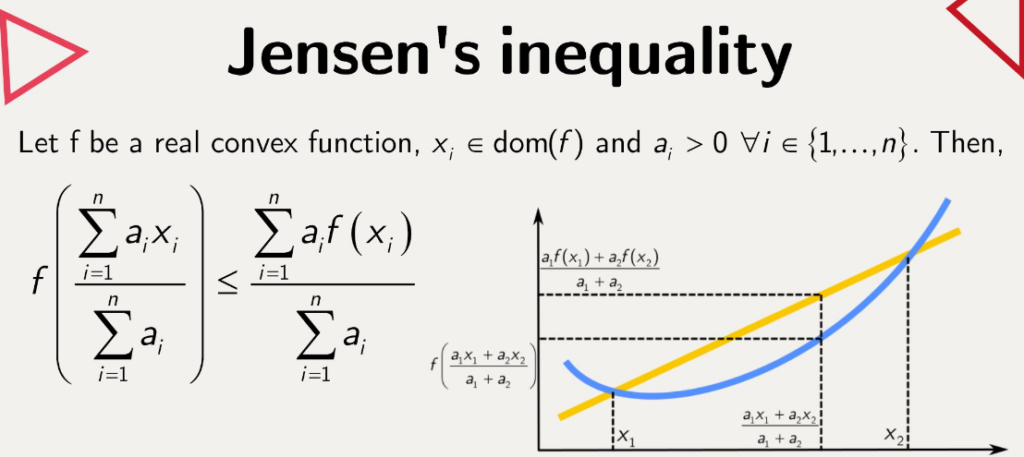
Jensen’s inequality says that if our function is convex (remember, it curves upwards), then the function of the weighted average of our numbers is less than or equal to the weighted average of the function of our numbers.
In other words, if we first average our numbers and then apply our function, we get a number that is less than to what we would get by first applying our function to each number and then averaging the results.
This might seem like a subtle point, but it’s actually very important in the areas of mathematics and economics. For example, it’s used in the theory of risk aversion, which says that people prefer a sure thing to a gamble with the same expected value. This is because the utility of the expected wealth level (which is a kind of average) is less than the expected utility of various wealth levels (which is the function of the wealth levels).
So, Jensen’s inequality is like a mathematical version of the saying “A bird in the hand is worth two in the bush”. It’s a way of saying that, when dealing with a convex function, it’s better to take the sure thing (the function of the average) than to gamble on the uncertain outcome (the average of the function).
Convex function: A function f: R → R is convex if it satisfies a certain property related to the line segment connecting any two points on the graph of the function.
Let’s take any two points x and y in the domain of the function. The line segment connecting the points (x, f(x)) and (y, f(y)) on the graph of the function is given by the equation:
This line segment is a weighted average of the function values f(x) and f(y), where the weights are t and (1-t), respectively. When t=0, we get L(t) = f(y), and when t=1, we get L(t) = f(x). For t between 0 and 1, L(t) gives us points on the line segment between (x, f(x)) and (y, f(y)).
Now, the function f is said to be convex if the value of the function at any point on the line segment connecting (x, f(x)) and (y, f(y)) is less than or equal to the corresponding point on the line segment itself. In other words, for all t in [0, 1], we must have:
This is the definition of a convex function. It’s a geometric property that says the graph of the function lies below the line segment connecting any two points on the graph. This property is what makes the function “bowed” or “curved” upwards, which is why it’s called convex.
Imagine you have a function f that represents a curve on a graph. Now, let’s pick two points on this curve, let’s call them point A and point B. Point A has coordinates (x, f(x)) and point B has coordinates (y, f(y)).
We want to draw a straight line segment that connects these two points. This line segment is a mix of points A and B, where the “mixing” is determined by a parameter “t” that ranges from 0 to 1.
When t=0, we’re fully at B. So, the line segment at t=0 is just the point B itself, which has coordinates (y, f(y)). When t=1, we’re fully at A, the line segment at t=1 is just the point A itself, which has coordinates (x, f(x)).
Now, what happens when t is between 0 and 1? In this case, we’re at some point on the line segment between A and B. We create a line segment that starts at point B and gradually moves towards point A as t increases.
To achieve this, we take a weighted average of the function values at points A and B. The weight for point A is t, and the weight for point B is (1-t). This means that as t increases, the weight for point A becomes larger, and the weight for point B becomes smaller.
So, for any value of t between 0 and 1, we can calculate the coordinates of the segment by taking a weighted average of the function values at points A and B. This line segment is denoted L(t) = tf(x) + (1-t)f(y).
By using this weighted average, we create a line segment that connects points A and B. As t increases from 0 to 1, the line segment gradually moves from point B towards point A.
The key idea here is that a convex function is the one where the function value at any point on the line segment connecting (x, f(x)) and (y, f(y)) is less than or equal to the function value at the corresponding point on the line segment L(t). In other words, the curve of the function lies below the line segment connecting A and B.
This property of convex functions is what gives them their characteristic “bowed” or “curved” shape. It ensures that the function values at any point on the line segment are always less than or equal to the corresponding point on the line segment.
Jensen’s inequality states that for a convex function f, the function’s value at the expectation of a random variable is less than or equal to the expectation of the function’s values at points specified by the random variable. Formally, if X is a random variable and f is a convex function, then f(E[X]) ≤ E[f(X)].
convex function. A function f: R → R is convex if for all x, y in R and for all t in [0, 1], we have:
let’s consider a random variable X with a finite number of outcomes x1, x2, …, xn occurring with probabilities p1, p2, …, pn, respectively. We have:
and
We want to show that f[X]) ≤ E[f(X)].
By applying the definition of convexity (equation 1) to the terms in the expectation E[X] (equation 2), we get:
But the right-hand side of this inequality is just E[f(X)] (equation 3). So we have:
It’s a beautiful result that relies on the simple geometric intuition behind convex functions


