
This series of articles is dedicated to understanding AI/ML and how it relates to Fx trading. Most articles in the ether focus on predicting a price and are almost useless when it comes to finding profitable trading strategies and hence thats the focus here.
I have been trading Fx for 20 years using both traditional statistical and chart analysis and AI/ML for the last 5 years or so. With a bachelor of engineering, masters and several certificates in Machine Learning I will share some of the pitfalls that took me years to learn and explain why its difficult, but not impossible, to make a system work.
In the first articles we:
1. Created the most basic “hello world” example. We gathered data, generated a model and measured our result. This formed our basis to build upon.
2. We use class weights to get our model “in the ball park” and possibly “slightly better than guessing” and improved our measurement.
3. In the 3rd article we peaked under the covers of Logistic Regression to find its limitations, looking for where we might go next.
4. We considered normalization and its impact, realizing our hypothesis maybe untrue.
5. A brief introduction into using other or new features and what impact they have.
6. This article reviews are measurement framework. Its our basis of comparison so needs to be right so we can compare model and feature combinations. We explore some of the pitfalls as this can get complicated
This is in no way financial advice and does not advocate for any specific trading strategy or suggest a profitable strategy is possible but instead is designed to help understand some of the details of the Fx market and how to apply ML techniques to it.
Firstly, lets recap our model.
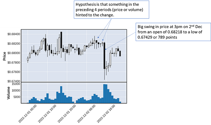
Our hypothesis is that something in the OHLC data of the preceding 4 periods predicts a sudden change of 200 points or more (we are measuring only “up” or “long” to make it simpler) in the next 4 periods. We have added class weights, different normalization techniques and multiple features, all without much success.

Our current measurement is using the typical logistic regression model (tp, fp, precision, recall, f1 etc.) and we subsequently discovered this wasn’t suitable (see previous articles).
While the metrics are good it only measures movement above 200 points. However, movement above 0 represents a profit. We are predicting a 200 points price change (in our training) but if the price moves 100 its still a win. So in article 2 (building on hello world) we modified our measurement algorithm to take that into account.
However, this too, doesn’t capture how Fx trading actually works.
I have known profession traders for many years and almost all of them use a take profit, and stop loss. This is to say they trade with a profit in mind and exit as soon as they hit it. The also have a maxmimum loss they will accept and exit when its reached. This can happen at any time, even if their hypothesis of movement is four hours ahead it can happen in the first, second or third period.

In the above chart above
Period 0 — Price moves up > 200 points (a win with a take profit in mind)
Point 1 — Price goes lower, back to roughly where it started
Period 2 — Price continues trend lower
Period 3 — Price is < -100 points (a loss)
Very few traders operate without a stop loss since it protects our account from massive falls by automatically trading out so the TP and SL need to be considered in our measurement of how successful we are.
We will assume (these will become meta parameters at a later point):
– We exit after a maximum of 4 periods (our prediction was 200 points after four periods and then exit at whatever the price is, that’s period 0, 1, 2, 3)
– A take profit of 200 points. If the price goes up 200 points at any time, we exit and take the profit
– A stop loss of -150 points. If the price goes down 150 points at any time, we will exit accepting a loss (to protect against the price might go down even further)
Each trader has their own method for profit and loss determination but the general rule is that since there are risks the upside has to be higher that then down side. There are rules of thumb around the “up side vs the down side” but we will cover them in a future article.
This effects two parts of our algorithm, the measurement AND the determination of y_true and we need to update both
This is our biggest change this article. We update how we measure y to include a stop loss and take profit. Then means changing our code to loop through each forward period looking in the “y range” (4 periods in our current hypothesis) checking for a stop loss or take profit. Note, it is possible a period could indicate both a stop loss and take profit, so we assume the stop loss (worst case for profit). Also, we now know the “points” that are actually moved limited by the stop loss, take profit or what it finished at the end, which will allow us to add a profit metric.
Note that:
– We added “date” to our features. We wont use this as a feature (yet) but for charting below.
– When considering the “Take Profit” we compare again the “high” price in the period.
– We considering the “Stop Loss” we compare against the “low” price in the period
– We now have the “points” moved (to determine a profit) and exit period (0, 1, 2 or 3 — for charting)
# create new holder for all values
x_values_df = pd.DataFrame()#
# X values look back
#
# loop thorugh feature name and "back periods" to go back
x_feature_names = []
for feature in feature_names:
for period in [1,2,3,4]:
# create the name (eg 'x_audusd_close_t-1')
feature_name = 'x_' + feature + '_t-' + str(period)
x_feature_names.append(feature_name)
x_values_df[feature_name] = df[feature].shift(period)
# Add "starting" values when used in normalization and date for reference
x_values_df['date'] = df['date']
x_values_df['x_audusd_open'] = df['audusd_open'].shift(4)
x_values_df['x_eurusd_open'] = df['eurusd_open'].shift(4)
x_values_df['audusd_open'] = df['audusd_open']
x_values_df['eurusd_open'] = df['eurusd_open']
#
# Y values look forward
#
# add all future y values for future periods
# set y=1 for >= 200 points
# set y=-1 for <= -150 (for later use)
# set y=0 for all else
# set y_points to actual points finished with (for later calculation of profit)
x_values_df['y'] = -2 # start wtih -2 to search for not -1,0,1
x_values_df['y_points'] = 0 # start with no point movement
for period in [0,1,2,3]: # loop thorugh each forward period in y (4 forward periods)
# names to store future price and change points
name = 'y_t-' + str(period) #name of future y value
price_name = 'y_change_price_' + str(period) # name of future y points change
points_name = 'y_change_points_' + str(period) # name of future y points change
# add important future values to spreadsheet
x_values_df[name] = df['audusd_close'].shift(-period)
x_values_df[name + '_low'] = df['audusd_low'].shift(-period)
x_values_df[name + '_high'] = df['audusd_high'].shift(-period)
# calculate change in points
x_values_df[price_name] = x_values_df[name] - df['audusd_open']
x_values_df[points_name] = x_values_df[price_name] * 100000
x_values_df[price_name + '_low'] = x_values_df[name + '_low'] - df['audusd_open']
x_values_df[points_name + '_low'] = x_values_df[price_name + '_low'] * 100000
x_values_df[price_name + '_high'] = x_values_df[name + '_high'] - df['audusd_open']
x_values_df[points_name + '_high'] = x_values_df[price_name + '_high'] * 100000
# get and calculate all "down" values where y isnt already set
# down "down" first, for case where bar goes both up and down in the same period assume down first (worst case for profit)
down_df = x_values_df[(x_values_df['y'] == -2) & (x_values_df[points_name + '_low'] <= -150)]
x_values_df.loc[down_df.index, 'y'] = -1
x_values_df.loc[down_df.index, 'y_points'] = -150
x_values_df.loc[down_df.index, 'y_finish_period'] = period
# get and calculate all "up" vales where y isnt already set
up_df = x_values_df[(x_values_df['y'] == -2) & (x_values_df[points_name + '_high'] >= 200)]
x_values_df.loc[up_df.index, 'y'] = 1
x_values_df.loc[up_df.index, 'y_points'] = 200
x_values_df.loc[up_df.index, 'y_finish_period'] = period
# if no period triggered tp/sl then no movement (y=0) and points are whatever it is at the end of the period
none_df = x_values_df[x_values_df['y'] == -2]
x_values_df.loc[none_df.index, 'y'] = 0
x_values_df.loc[none_df.index, 'y_points'] = x_values_df[points_name]
x_values_df.loc[none_df.index, 'y_finish_period'] = 3
# set down (currently -1) to 0 since we arent using it (yet - we will later)
x_values_df.loc[x_values_df[x_values_df['y'] == -1].index, 'y'] = 0
# if points exceeds tp or sl then reset to sl/tp since these limits are fixed in trading
x_values_df.loc[x_values_df['y_points'] < -150, 'y_points'] = -150
x_values_df.loc[x_values_df['y_points'] > 200, 'y_points'] = 200
# and reset df (avoids indexing complications later) and done
x_values_df = x_values_df.copy()
return x_values_df, x_feature_names
Our y variable is updated above and flows through the code already in place so or measurement algorithm will work unchanged. However, because we now have a “points” metric we can check our effective profit. This is a pretty simple change to our measurement algorithm.
A few notes:
- We have simplified our divide using the numpy divide function which automatically takes care of divide by 0.
- We have added a “profit” metric which is the cumulative points. Remember we have a 200 points take profit and 150 point stop loss. (so our potential profit is higher than our potential loss).
def divide(a, b):a = np.asarray(a).astype(float)
b = np.asarray(b).astype(float)
result = np.divide(a, b, out=np.zeros_like(a), where=b != 0)
return result
def show_metrics(lr, x, y_true, y_points, display=True):
x = x.to_numpy()
y_true = y_true.to_numpy()
y_points = y_points.to_numpy()
# predict from teh val set meas we have predictions and true values as binaries
y_pred = lr.predict(x)
#basic error types
log_loss_error = log_loss(y_true, y_pred)
score = lr.score(x, y_true)
#
# Customized metrics to confusion matrix
#
tp = np.where((y_pred == 1) & (y_points >= 0), 1, 0).sum()
fp = np.where((y_pred == 1) & (y_points < 0), 1, 0).sum()
tn = np.where((y_pred == 0) & (y_points < 0), 1, 0).sum()
fn = np.where((y_pred == 0) & (y_points >= 0), 1, 0).sum()
# derived from confusion matrix
precision = float(divide(tp, (tp+fp)))
recall = float(divide(tp, (tp + fn)))
f1 = float(divide((precision*recall), (precision + recall)))
# profit calculation (if predicted use points, otherwise 0)
profit = np.where(y_pred==1, y_points, 0).sum()
# output the errors
if display:
print('Errors Loss: {:.4f}'.format(log_loss_error))
print('Errors Score: {:.2f}%'.format(score*100))
print('Errors tp: {} ({:.2f}%)'.format(tp, tp/len(y_val)*100))
print('Errors fp: {} ({:.2f}%)'.format(fp, fp/len(y_val)*100))
print('Errors tn: {} ({:.2f}%)'.format(tn, tn/len(y_val)*100))
print('Errors fn: {} ({:.2f}%)'.format(fn, fn/len(y_val)*100))
print('Errors Precision: {:.2f}%'.format(precision*100))
print('Errors Recall: {:.2f}%'.format(recall*100))
print('Errors F1: {:.2f}'.format(f1*100))
print('profit: {:.2f} points'.format(profit))
errors = {
'loss': log_loss_error,
'score': score,
'tp': tp,
'fp': fp,
'tn': tn,
'fn': fn,
'precision': precision,
'recall': recall,
'f1': f1,
'profit': profit
}
return errors
Firstly, lets add some code to calculate the “profit” (effectively a trade by trade calculation) and then to chart each trade so we can visualize what’s going on and check it makes sense.
def get_trades(lr, x, y_change_points):y_pred = lr.predict(x)
trades = []
for ix in range(len(y_pred)):
if y_pred[ix] == 1:
won = False
profit = y_change_points.iloc[ix]
if profit > 0:
won = True
trades.append([ix, won, profit])
trades_df = pd.DataFrame(trades, columns=['ix', 'won', 'profit'])
return trades_df
def chart_trades(trades, features_df, raw_df, number_of_charts):
rows = math.ceil(number_of_charts / 3)
fig, axes = plt.subplots(nrows=rows, ncols=3)
for chart_ix in range(number_of_charts):
# get indexes and ate for chart
trade_ix = random.randint(0, len(trades))
data_ix = trades['ix'].iloc[trade_ix] + 35373
date = features_df['date'].iloc[data_ix]
# prepard data for OHLC candles
mpf_df = pd.DataFrame()
mpf_df[['date', 'Open', 'High', 'Low', 'Close', 'Volume']] =
raw_df[['date', 'audusd_open', 'audusd_high', 'audusd_low', 'audusd_close', 'audusd_volume']]
.iloc[data_ix-4:data_ix+4].to_numpy()
mpf_df['date'] = pd.to_datetime(mpf_df['date'])
mpf_df = mpf_df.set_index('date')
mpf_df = mpf_df[['Open', 'High', 'Low', 'Close', 'Volume']].astype(float)
# plot the chart
ax = axes.flatten()[chart_ix]
mpf.plot(mpf_df, ax=ax, volume=False, datetime_format='', type='candle')
# add title
ax.set_title(date.strftime('%d-%m-%Y %H:%M'))
# add marker to seperate history and future
ax.plot([4, 4], [mpf_df['High'].iloc[4], ax.get_ylim()[1]], color='y', marker='o', linewidth=3.0)
ax.plot([4, 4], [ax.get_ylim()[0], mpf_df['Low'].iloc[4]], color='y', marker='o', linewidth=3.0)
# horizontal lines indicator tp and sl
open_price = mpf_df['Open'].iloc[4]
ax.axhline(open_price+(200/100000), color='green', linewidth=1.5)
ax.axhline(open_price-(150/100000), color='red', linewidth=1.5)
# plot line from start to close position
close_period = int(features_df['y_finish_period'].iloc[data_ix])
profit = features_df['y_points'].iloc[data_ix]
close_price = open_price + (profit / 100000)
ax.plot([4,4+close_period], [mpf_df['Open'].iloc[4], close_price], color='r', marker='x', linewidth=1.5)
# text box indicating result
txt = 'Win: {}nProfit: {:.2f}nExit: {}'.format(trades.iloc[trade_ix]['won'], trades.iloc[trade_ix]['profit'], close_period)
props = dict(boxstyle='round', facecolor='wheat', alpha=0.5)
ax.text(0.05, 0.75, txt, style='italic', transform=ax.transAxes, size=10, bbox=props)
plt.show()
return

This type of visualization exercise is very useful and I always recommend it. It will help you “see” what’s going on, check your charts carefully and if anything doesn’t make sense go back and figure out why, its likely you have some mistakes somewhere.
Now we can run our testing algorithm and update the metrics.
#
# Main loop to test different normalization techniques
#
for norm_method in ['price', 'points', 'percentage', 'minmax', 'stddev']:# load raw data
raw_df = load_data()
# create features
feature_names =['audusd_open', 'audusd_close', 'audusd_high', 'audusd_low', 'audusd_volume',
'eurusd_open', 'eurusd_close', 'eurusd_high', 'eurusd_low', 'eurusd_volume']
df, x_feature_names = create_xy_values(raw_df, feature_names)
# prepare data for learning (normalize, split and class weights)
norm_df, x_feature_names_norm = normalize_data(df, x_feature_names, method=norm_method)
x_train, y_train, x_val, y_val, y_val_change_points, no_train_samples = get_train_val(norm_df, x_feature_names_norm)
class_weights = get_class_weights(y_train, display=False)
# train the model
lr = LogisticRegression(class_weight=class_weights, max_iter=1000)
lr.fit(x_train, y_train)
# if we want to see all actual trades and chart them
trades_df = get_trades(lr, x_val, y_val_change_points)
print('trades {}, wins {}, profit {:.2f}'.format(len(trades_df), trades_df['won'].sum(), trades_df['profit'].sum()))
# if we want to chart trades
chart_trades(trades_df, df, raw_df, number_of_charts=9)
# to show standard errors
print('Errrors for method {}'.format(norm_method))
errors = show_metrics(lr, x_val, y_val, y_val_change_points, display=True)

We immediately can see that the model performance has deteriated and the trading losses would be substantial. This raises a few questions:
1. Why has the model performance deteriorated?
The precisions are not quite low (approx 43%) which is well below guessing. We have done two things. By considering a TP/SL have added another step disconnecting the result Y and whats actually happening. We also have a large number of features which logistic regression will struggle to deal with.
2. Why are the trading losses so large?
This is easier to see by calculating how many bars go up vs down.
def check_simultaneous_sl_tp(trades_df, features_df, raw_df):trade_ixs = trades_df['ix'].tolist()
results = []
for ix in range(35373, len(features_df)):
low = raw_df['audusd_low'].iloc[ix]
high = raw_df['audusd_high'].iloc[ix]
open = raw_df['audusd_open'].iloc[ix]
points_high = round((high - open) * 100000, 2)
points_low = round((low - open) * 100000, 2)
gone_high, gone_low, during_trade = False, False, False
if points_high > 200:
gone_high = True
if points_low < -150:
gone_low = True
if (ix-35373) in trade_ixs:
during_trade = True
results.append([ix, gone_high, gone_low, during_trade])
results_df = pd.DataFrame(results, columns=['ix', 'high', 'low', 'trade'])
print('Total Periods {}'.format(len(results_df)))
print('Highs {}'.format(len(results_df[results_df['high'] == True])))
print('Lows {}'.format(len(results_df[results_df['low'] == True])))
print('Trades {}'.format(len(results_df[results_df['trade'] == True])))
print('Not In Trade Highs AND Lows together {}'.format(len(results_df[(results_df['high'] == True) & (results_df['low'] == True)])))
print('In Trade Highs AND Lows together {}'.format(len(results_df[(results_df['high'] == True) & (results_df['low'] == True) & (results_df['trade'] == True)])))
return results_df
Total Periods 15161
Highs 787
Lows 1743
Trades 5087
Not In Trade Highs AND Lows together 43
In Trade Highs AND Lows together 29
We can see there are far more “down” movement than up and 29 trades have > TP and < SL in the same period (we assume the SL but actually don’t know which way it went).
The debugging is getting a little more complicated so I have actually moved to VS Code which provides, in my opinion, easier debugging capability to colab. I advise you check it out but I will continue to post updates in colab.
Its extremely import you check and recheck your calculations. Remember Garbage In — Garbage Out! Check, double check and triple check. If you get your input data wrong (the x or y) you will never make it work or you will find it does work in training but not practice and result in trading losses.
Updating the measurement to include Stop Loss and Take Profits made our model worse but we will need to incorporate it as its an important part of Fx trading.
Using the model “as is”, our trading loss would be substantial.
There are a few directions we can go. We can work on our optimizing our meta parameters (like stop loss, take profit, normalization method etc.) or we can work on our precision which is worse then guessing. This is direction we will take (notice I talk about the metric we are trying to improve, not a specific technique to do it).
Next article we will focus on improving our precision with new derived features and some more feature engineering.


