
A Machine Learning case study
by Irene Rivero (13/01/2023)
This project is about building a K-mean unsupervised machine learning algorithm in Scikit-Learn to perform customer segmentation. We will complete the following tasks:
- Understand the problem statement and the business case
- Import libraries and datasets
- Visualize and explore datasets
- Use Scikit-Learn library to find the optimal number of clusters using elbow method
- Apply k-means using Scikit-Learn to perform customer segmentation
- Apply Principal Component Analysis (PCA) technique to perform dimensionality reduction and data visualization
K-means intuition
K-means is an unsupervised learning algorithm (clustering). It works by grouping some data points together (clustering) in an unsupervised fashion.
The algorithm groups observations with similar attribute values together by measuring the Euclidian distance between points.

K-means algorithm steps:
- Choose number of clusters “K”
- Select random K points that are going to be the centroids for each cluster
- Assign each data point to the nearest centroid, doing so will enable us to create “K” number of clusters
- Calculate a new centroid for each cluster
- Reassign each data point to the new closest centroid
- Go to step 4 and repeat

Understand the problem statement and the business case
In this project, I will act as if I was hired as a data scientist at a bank. I have been provided with extensive data on the bank’s customers for the past six months.
Data includes transactions, frequency, amount, tenure…
The bank marketing team would like to leverage AI/ML to launch a targeted marketing ad campaign that is tailored to specific group of customers.
In order for this campaign to be successful, the bank has to divide its customers into at least 3 distinctive groups.
This process is known as “marketing segmentation” and it is crucial for maximizing marketing campaign conversion rate.
There will be four types of groups of customers:
Transactors: Customers who pay the least amount of interest charges and are careful with their money.
Revolvers: Customers who use their credit card as a loan. This group is the most lucrative sector for the bank since they pay 20%+ interest.
New customers: This customers with low tenure can be targeted to enroll in other bank services (ex: travel credit card).
VIP/Prime: Customers with high credit limit/% of full payment; targeted to increase their credit limit/ spending.
Data Source: https://www.kaggle.com/arjunbhasin2013/ccdata
Import libraries and datasets
!pip install jupyterthemes
import jupyterthemes
import pandas as pd
import numpy as np
import seaborn as sns
import matplotlib.pyplot as plt
from sklearn.preprocessing import StandardScaler, normalize
from sklearn.cluster import KMeans
from sklearn.decomposition import PCA
from jupyterthemes import jtplot
jtplot.style(theme='monokai', context='notebook', ticks=True, grid=False)
# setting the style of the notebook to be monokai theme
# this line of code is important to ensure that we are able to see the x and y axes clearly
# You have to include the full link to the csv file containing your dataset
creditcard_df = pd.read_csv('.../Unsupervised Machine Learning for Customer Segmentation/marketing_data.csv')# CUSTID: Identification of Credit Card holder
# BALANCE: Balance amount left in customer's account to make purchases
# BALANCE_FREQUENCY: How frequently the Balance is updated, score between 0 and 1 (1 = frequently updated, 0 = not frequently updated)
# PURCHASES: Amount of purchases made from account
# ONEOFFPURCHASES: Maximum purchase amount done in one-go
# INSTALLMENTS_PURCHASES: Amount of purchase done in installment
# CASH_ADVANCE: Cash in advance given by the user
# PURCHASES_FREQUENCY: How frequently the Purchases are being made, score between 0 and 1 (1 = frequently purchased, 0 = not frequently purchased)
# ONEOFF_PURCHASES_FREQUENCY: How frequently Purchases are happening in one-go (1 = frequently purchased, 0 = not frequently purchased)
# PURCHASES_INSTALLMENTS_FREQUENCY: How frequently purchases in installments are being done (1 = frequently done, 0 = not frequently done)
# CASH_ADVANCE_FREQUENCY: How frequently the cash in advance being paid
# CASH_ADVANCE_TRX: Number of Transactions made with "Cash in Advance"
# PURCHASES_TRX: Number of purchase transactions made
# CREDIT_LIMIT: Limit of Credit Card for user
# PAYMENTS: Amount of Payment done by user
# MINIMUM_PAYMENTS: Minimum amount of payments made by user
# PRC_FULL_PAYMENT: Percent of full payment paid by user
# TENURE: Tenure of credit card service for user
creditcard_df

creditcard_df.info()
# Let's apply info and get additional insights on our dataframe
# 18 features with 8950 points  <class 'pandas.core.frame.DataFrame'>
RangeIndex: 8950 entries, 0 to 8949
Data columns (total 17 columns):
#   Column                            Non-Null Count  Dtype
---  ------                            --------------  -----
0   BALANCE                           8950 non-null   float64
1   BALANCE_FREQUENCY                 8950 non-null   float64
2   PURCHASES                         8950 non-null   float64
3   ONEOFF_PURCHASES                  8950 non-null   float64
4   INSTALLMENTS_PURCHASES            8950 non-null   float64
5   CASH_ADVANCE                      8950 non-null   float64
6   PURCHASES_FREQUENCY               8950 non-null   float64
7   ONEOFF_PURCHASES_FREQUENCY        8950 non-null   float64
8   PURCHASES_INSTALLMENTS_FREQUENCY  8950 non-null   float64
9   CASH_ADVANCE_FREQUENCY            8950 non-null   float64
10  CASH_ADVANCE_TRX                  8950 non-null   int64
11  PURCHASES_TRX                     8950 non-null   int64
12  CREDIT_LIMIT                      8950 non-null   float64
13  PAYMENTS                          8950 non-null   float64
14  MINIMUM_PAYMENTS                  8950 non-null   float64
15  PRC_FULL_PAYMENT                  8950 non-null   float64
16  TENURE                            8950 non-null   int64
dtypes: float64(14), int64(3)
memory usage: 1.2 MB
What is the average, minimum and maximum “BALANCE” amount?
print('Average, min, max =', creditcard_df['BALANCE'].mean(), creditcard_df['BALANCE'].min(), creditcard_df['BALANCE'].max() )Average, min, max = 1564.4748276781006 0.0 19043.13856
# Let's apply describe() and get more statistical insights on our dataframe
# Mean balance is $1564
# Balance frequency is frequently updated on average ~0.9
# Purchases average is $1000
# one off purchase average is ~$600
# Average purchases frequency is around 0.5
# average ONEOFF_PURCHASES_FREQUENCY, PURCHASES_INSTALLMENTS_FREQUENCY, and CASH_ADVANCE_FREQUENCY are generally low
# Average credit limit ~ 4500
# Percent of full payment is 15%
# Average tenure is 11 yearscreditcard_df.describe()

Obtaining the features of the customer who made the maximum “ONEOFF_PURCHASES”
creditcard_df[creditcard_df['ONEOFF_PURCHASES'] == 40761.25]

What about the customer with the maximum “CASH_ADVANCE”.
creditcard_df['CASH_ADVANCE'].max()47137.21176
creditcard_df[creditcard_df['CASH_ADVANCE'] == 47137.21176]

Visualize and explore datasets
# Let's see if we have any missing data? luckily we don't have many!
sns.heatmap(creditcard_df.isnull(), yticklabels = False, cbar = False, cmap="Blues")

creditcard_df.isnull().sum()CUST_ID                               0
BALANCE                               0
BALANCE_FREQUENCY                     0
PURCHASES                             0
ONEOFF_PURCHASES                      0
INSTALLMENTS_PURCHASES                0
CASH_ADVANCE                          0
PURCHASES_FREQUENCY                   0
ONEOFF_PURCHASES_FREQUENCY            0
PURCHASES_INSTALLMENTS_FREQUENCY      0
CASH_ADVANCE_FREQUENCY                0
CASH_ADVANCE_TRX                      0
PURCHASES_TRX                         0
CREDIT_LIMIT                          1
PAYMENTS                              0
MINIMUM_PAYMENTS                    313
PRC_FULL_PAYMENT                      0
TENURE                                0
dtype: int64
# Fill up the missing elements with mean of the 'MINIMUM_PAYMENT'
creditcard_df.loc[(creditcard_df['MINIMUM_PAYMENTS'].isnull() == True), 'MINIMUM_PAYMENTS'] = creditcard_df['MINIMUM_PAYMENTS'].mean()
creditcard_df.isnull().sum()CUST_ID                             0
BALANCE                             0
BALANCE_FREQUENCY                   0
PURCHASES                           0
ONEOFF_PURCHASES                    0
INSTALLMENTS_PURCHASES              0
CASH_ADVANCE                        0
PURCHASES_FREQUENCY                 0
ONEOFF_PURCHASES_FREQUENCY          0
PURCHASES_INSTALLMENTS_FREQUENCY    0
CASH_ADVANCE_FREQUENCY              0
CASH_ADVANCE_TRX                    0
PURCHASES_TRX                       0
CREDIT_LIMIT                        1
PAYMENTS                            0
MINIMUM_PAYMENTS                    0
PRC_FULL_PAYMENT                    0
TENURE                              0
dtype: int64
#Fill out missing elements in the CREDIT_LIMIT column
#Double check and make sure that no missing elements are presentcreditcard_df.loc[(creditcard_df['CREDIT_LIMIT'].isnull() == True), 'CREDIT_LIMIT'] = creditcard_df['CREDIT_LIMIT'].mean()
creditcard_df.isnull().sum()
CUST_ID 0
BALANCE 0
BALANCE_FREQUENCY 0
PURCHASES 0
ONEOFF_PURCHASES 0
INSTALLMENTS_PURCHASES 0
CASH_ADVANCE 0
PURCHASES_FREQUENCY 0
ONEOFF_PURCHASES_FREQUENCY 0
PURCHASES_INSTALLMENTS_FREQUENCY 0
CASH_ADVANCE_FREQUENCY 0
CASH_ADVANCE_TRX 0
PURCHASES_TRX 0
CREDIT_LIMIT 0
PAYMENTS 0
MINIMUM_PAYMENTS 0
PRC_FULL_PAYMENT 0
TENURE 0
dtype: int64
sns.heatmap(creditcard_df.isnull(), yticklabels = False, cbar = False, cmap="Blues")

# Let's see if we have duplicated entries in the data
creditcard_df.duplicated().sum()0
#Drop Customer ID column 'CUST_ID' and make sure that the column has been removed from the dataframe
creditcard_df.drop('CUST_ID', axis=1, inplace= True)creditcard_df.info()
<class 'pandas.core.frame.DataFrame'>
RangeIndex: 8950 entries, 0 to 8949
Data columns (total 17 columns):
#   Column                            Non-Null Count  Dtype
---  ------                            --------------  -----
0   BALANCE                           8950 non-null   float64
1   BALANCE_FREQUENCY                 8950 non-null   float64
2   PURCHASES                         8950 non-null   float64
3   ONEOFF_PURCHASES                  8950 non-null   float64
4   INSTALLMENTS_PURCHASES            8950 non-null   float64
5   CASH_ADVANCE                      8950 non-null   float64
6   PURCHASES_FREQUENCY               8950 non-null   float64
7   ONEOFF_PURCHASES_FREQUENCY        8950 non-null   float64
8   PURCHASES_INSTALLMENTS_FREQUENCY  8950 non-null   float64
9   CASH_ADVANCE_FREQUENCY            8950 non-null   float64
10  CASH_ADVANCE_TRX                  8950 non-null   int64
11  PURCHASES_TRX                     8950 non-null   int64
12  CREDIT_LIMIT                      8950 non-null   float64
13  PAYMENTS                          8950 non-null   float64
14  MINIMUM_PAYMENTS                  8950 non-null   float64
15  PRC_FULL_PAYMENT                  8950 non-null   float64
16  TENURE                            8950 non-null   int64
dtypes: float64(14), int64(3)
memory usage: 1.2 MB
n = len(creditcard_df.columns)
n17
creditcard_df.columnsIndex(['BALANCE', 'BALANCE_FREQUENCY', 'PURCHASES', 'ONEOFF_PURCHASES',
'INSTALLMENTS_PURCHASES', 'CASH_ADVANCE', 'PURCHASES_FREQUENCY',
'ONEOFF_PURCHASES_FREQUENCY', 'PURCHASES_INSTALLMENTS_FREQUENCY',
'CASH_ADVANCE_FREQUENCY', 'CASH_ADVANCE_TRX', 'PURCHASES_TRX',
'CREDIT_LIMIT', 'PAYMENTS', 'MINIMUM_PAYMENTS', 'PRC_FULL_PAYMENT',
'TENURE'],
dtype='object')
# distplot combines the matplotlib.hist function with seaborn kdeplot()
# KDE Plot represents the Kernel Density Estimate
# KDE is used for visualizing the Probability Density of a continuous variable.
# KDE demonstrates the probability density at different values in a continuous variable. # Mean of balance is $1500
# 'Balance_Frequency' for most customers is updated frequently ~1
# For 'PURCHASES_FREQUENCY', there are two distinct group of customers
# For 'ONEOFF_PURCHASES_FREQUENCY' and 'PURCHASES_INSTALLMENT_FREQUENCY' most users don't do one off puchases or installment purchases frequently
# Very small number of customers pay their balance in full 'PRC_FULL_PAYMENT'~0
# Credit limit average is around $4500
# Most customers are ~11 years tenure
plt.figure(figsize=(10,50))
for i in range(len(creditcard_df.columns)):
plt.subplot(17, 1, i+1)
sns.distplot(creditcard_df[creditcard_df.columns[i]], kde_kws={"color": "b", "lw": 3, "label": "KDE"}, hist_kws={"color": "g"})
plt.title(creditcard_df.columns[i])
plt.tight_layout()

Obtaining the correlation matrix between features.
correlations = creditcard_df.corr()
f, ax = plt.subplots(figsize = (20, 10))
sns.heatmap(correlations, annot = True)

Use Scikit-Learn library to find the optimal number of clusters using elbow method
The elbow method is a heuristic method of interpretation and validation of consistency within cluster analysis designed to help find the appropriate number of clusters in a dataset.
If the line chart looks like an arm, then the “elbow” on the arm is the value of k that is the best.
# Let's scale the data first
scaler = StandardScaler()
creditcard_df_scaled = scaler.fit_transform(creditcard_df)creditcard_df_scaled.shape
(8950, 17)
creditcard_df_scaled
array([[-0.73198937, -0.24943448, -0.42489974, ..., -0.31096755,
-0.52555097, 0.36067954],
[ 0.78696085, 0.13432467, -0.46955188, ..., 0.08931021,
0.2342269 , 0.36067954],
[ 0.44713513, 0.51808382, -0.10766823, ..., -0.10166318,
-0.52555097, 0.36067954],
...,
[-0.7403981 , -0.18547673, -0.40196519, ..., -0.33546549,
0.32919999, -4.12276757],
[-0.74517423, -0.18547673, -0.46955188, ..., -0.34690648,
0.32919999, -4.12276757],
[-0.57257511, -0.88903307, 0.04214581, ..., -0.33294642,
-0.52555097, -4.12276757]])
# Index(['BALANCE', 'BALANCE_FREQUENCY', 'PURCHASES', 'ONEOFF_PURCHASES',
# 'INSTALLMENTS_PURCHASES', 'CASH_ADVANCE', 'PURCHASES_FREQUENCY',
# 'ONEOFF_PURCHASES_FREQUENCY', 'PURCHASES_INSTALLMENTS_FREQUENCY',
# 'CASH_ADVANCE_FREQUENCY', 'CASH_ADVANCE_TRX', 'PURCHASES_TRX',
# 'CREDIT_LIMIT', 'PAYMENTS', 'MINIMUM_PAYMENTS', 'PRC_FULL_PAYMENT',
# 'TENURE'], dtype='object')scores_1 = []
range_values= range (1, 20)
for i in range_values:
kmeans = KMeans(n_clusters= i)
kmeans.fit(creditcard_df_scaled)
scores_1.append(kmeans.inertia_)
plt.plot(scores_1, 'bx-')
# From this we can observe that, 4th cluster seems to be forming the elbow of the curve.
# However, the values does not reduce linearly until 8th cluster.
# Let's choose the number of clusters to be 7 or 8.

Apply k-means using Scikit-Learn to perform customer segmentation
kmeans = KMeans(7)
kmeans.fit(creditcard_df_scaled)
labels = kmeans.labels_ # labels (cluster) associated to each data point
kmeans.cluster_centers_.shape
(7, 17)
#create the dataframe that consists on the kmeans.cluster_centers_cluster_centers = pd.DataFrame(data = kmeans.cluster_centers_, columns = [creditcard_df.columns])
cluster_centers

# In order to understand what these numbers mean, let's perform inverse transformation
cluster_centers = scaler.inverse_transform(cluster_centers)
cluster_centers = pd.DataFrame(data = cluster_centers, columns = [creditcard_df.columns])
cluster_centers# First Customers cluster (Transactors): Those are customers who pay least amount of intrerest charges and careful with their money, Cluster with lowest balance ($104) and cash advance ($303), Percentage of full payment = 23%
# Second customers cluster (revolvers) who use credit card as a loan (most lucrative sector): highest balance ($5000) and cash advance (~$5000), low purchase frequency, high cash advance frequency (0.5), high cash advance transactions (16) and low percentage of full payment (3%)
# Third customer cluster (VIP/Prime): high credit limit $16K and highest percentage of full payment, target for increase credit limit and increase spending habits
# Fourth customer cluster (low tenure): these are customers with low tenure (7 years), low balance

labels.shape # Labels associated to each data point
(8950,)labels.max()
6
labels.min()
0
y_kmeans = kmeans.fit_predict(creditcard_df_scaled)
y_kmeans
array([6, 2, 0, ..., 5, 5, 5], dtype=int32)# concatenate the clusters labels to our original dataframe
creditcard_df_cluster = pd.concat([creditcard_df, pd.DataFrame({'cluster':labels})], axis = 1)
creditcard_df_cluster.head()

# Plot the histogram of various clusters
for i in creditcard_df.columns:
plt.figure(figsize = (35, 5))
for j in range(7):
plt.subplot(1,7,j+1)
cluster = creditcard_df_cluster[creditcard_df_cluster['cluster'] == j]
cluster[i].hist(bins = 20)
plt.title('{}    nCluster {} '.format(i,j))plt.show()


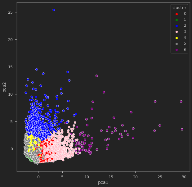
Apply Principal Component Analysis (PCA) technique to perform dimensionality reduction and data visualization
# Obtain the principal components
pca = PCA(n_components=2)
principal_comp = pca.fit_transform(creditcard_df_scaled)
principal_comp
array([[-1.6822199 , -1.07644877],
[-1.13829078,  2.5064681 ],
[ 0.96968555, -0.38353756],
...,
[-0.92620432, -1.8107839 ],
[-2.33655655, -0.65793819],
[-0.55642671, -0.40044766]])# Create a dataframe with the two components
pca_df = pd.DataFrame(data = principal_comp, columns =['pca1','pca2'])
pca_df.head()

# Concatenate the clusters labels to the dataframe
pca_df = pd.concat([pca_df,pd.DataFrame({'cluster':labels})], axis = 1)
pca_df.head()

ax = sns.scatterplot(x="pca1", y="pca2", hue = "cluster", data = pca_df, palette =['red','green','blue','pink','yellow','gray','purple'])


